MAR 536 Lab 8: plotting spatial data
2025-04-02
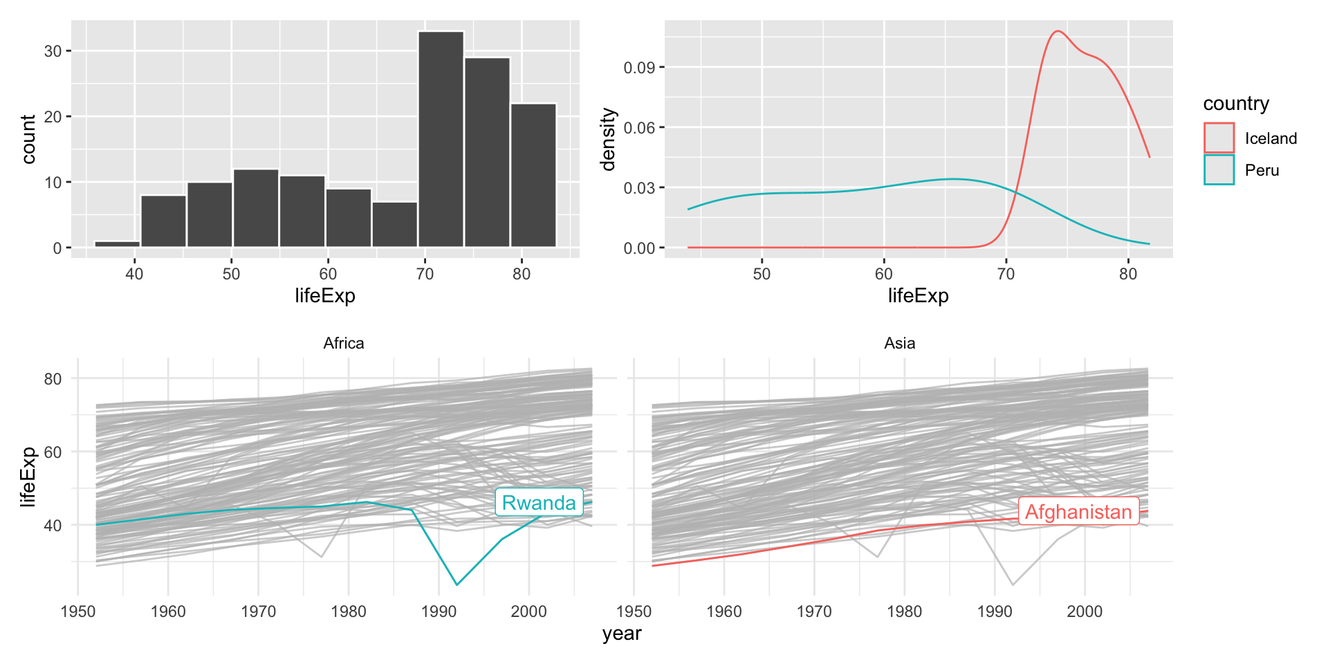
facet_grid()
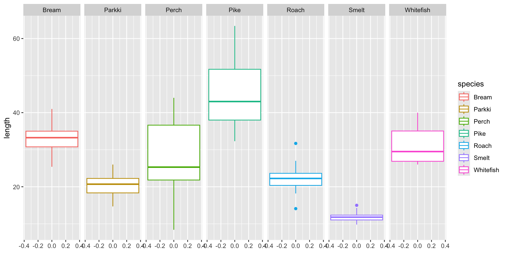
facet_grid()
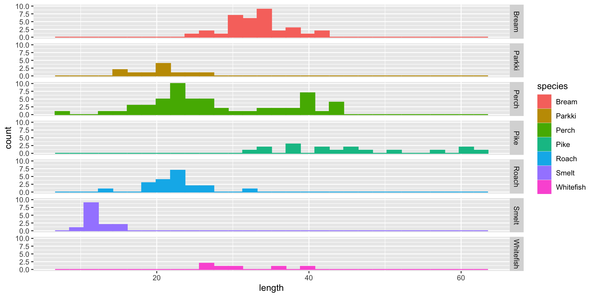
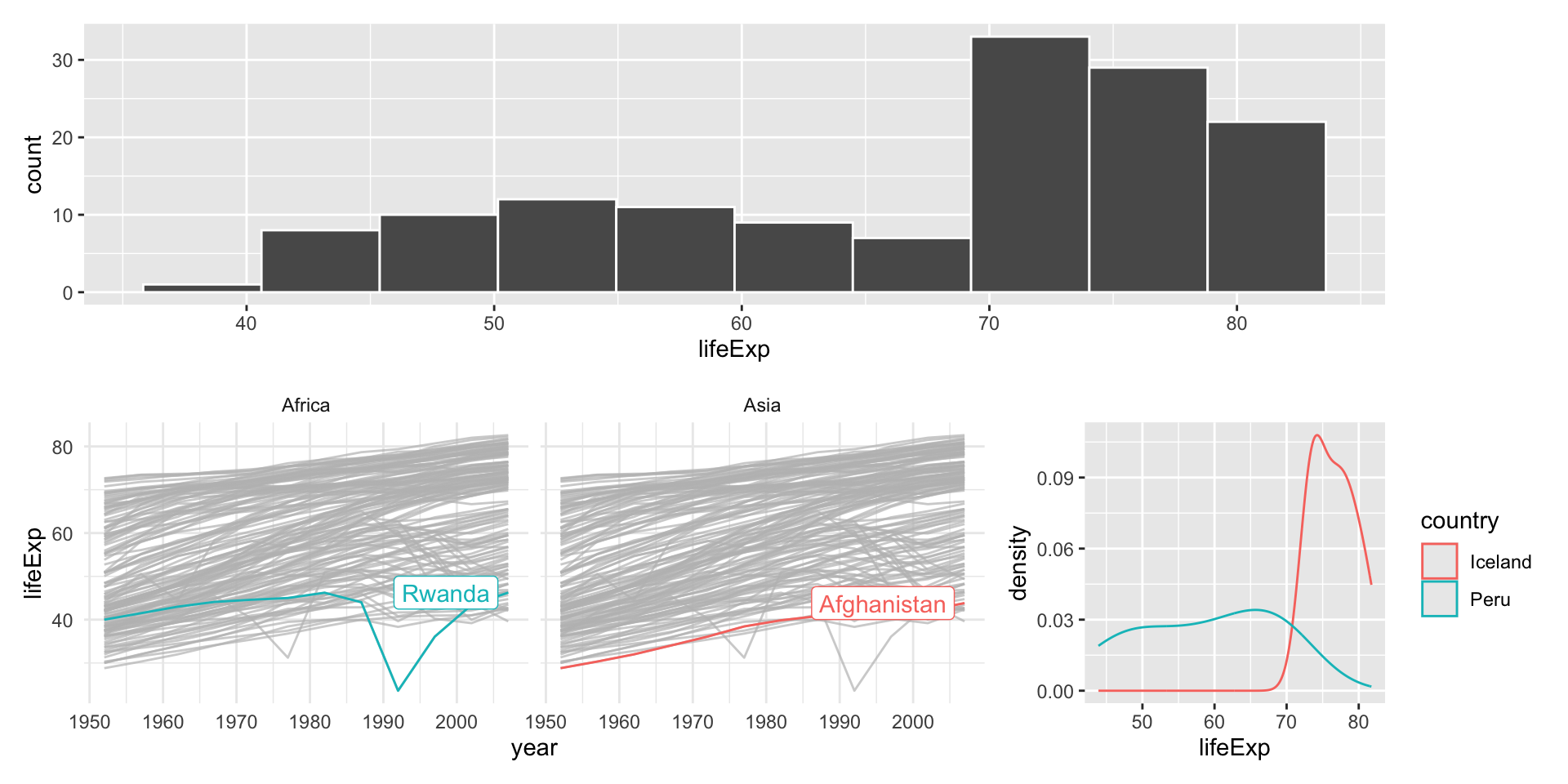
Some gapminder example plots to work with:
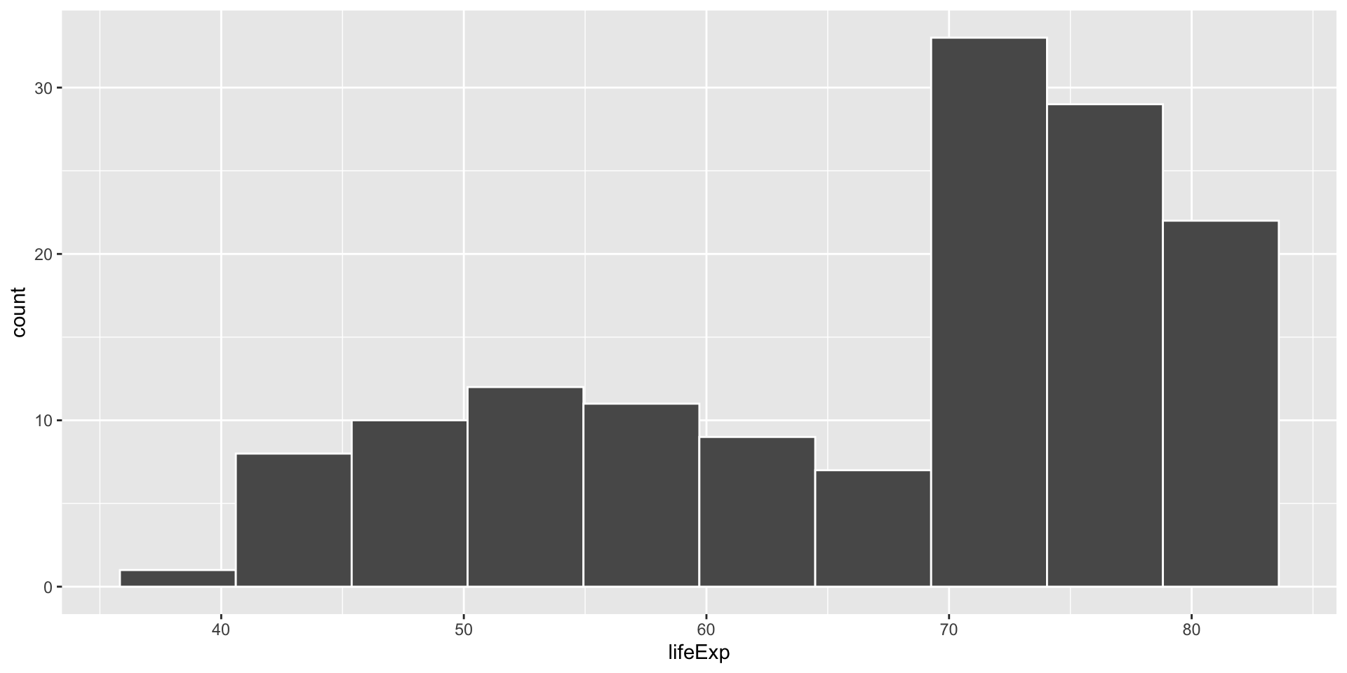
continents with low life expectancy
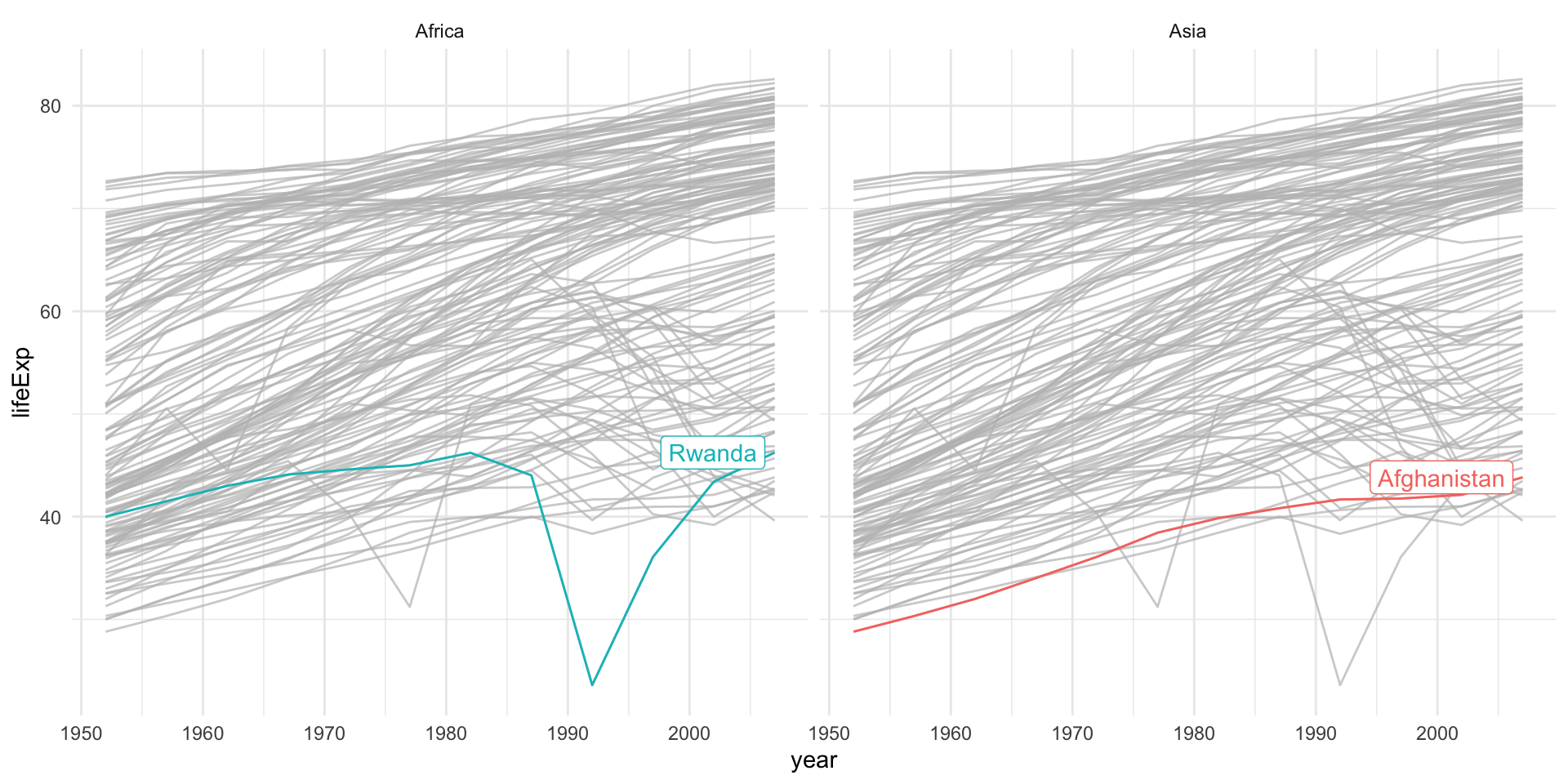
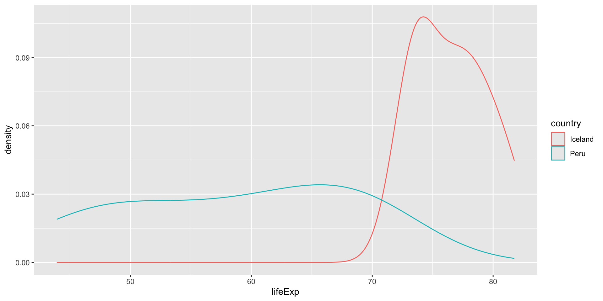
distribution of life expectancy over years for two countries
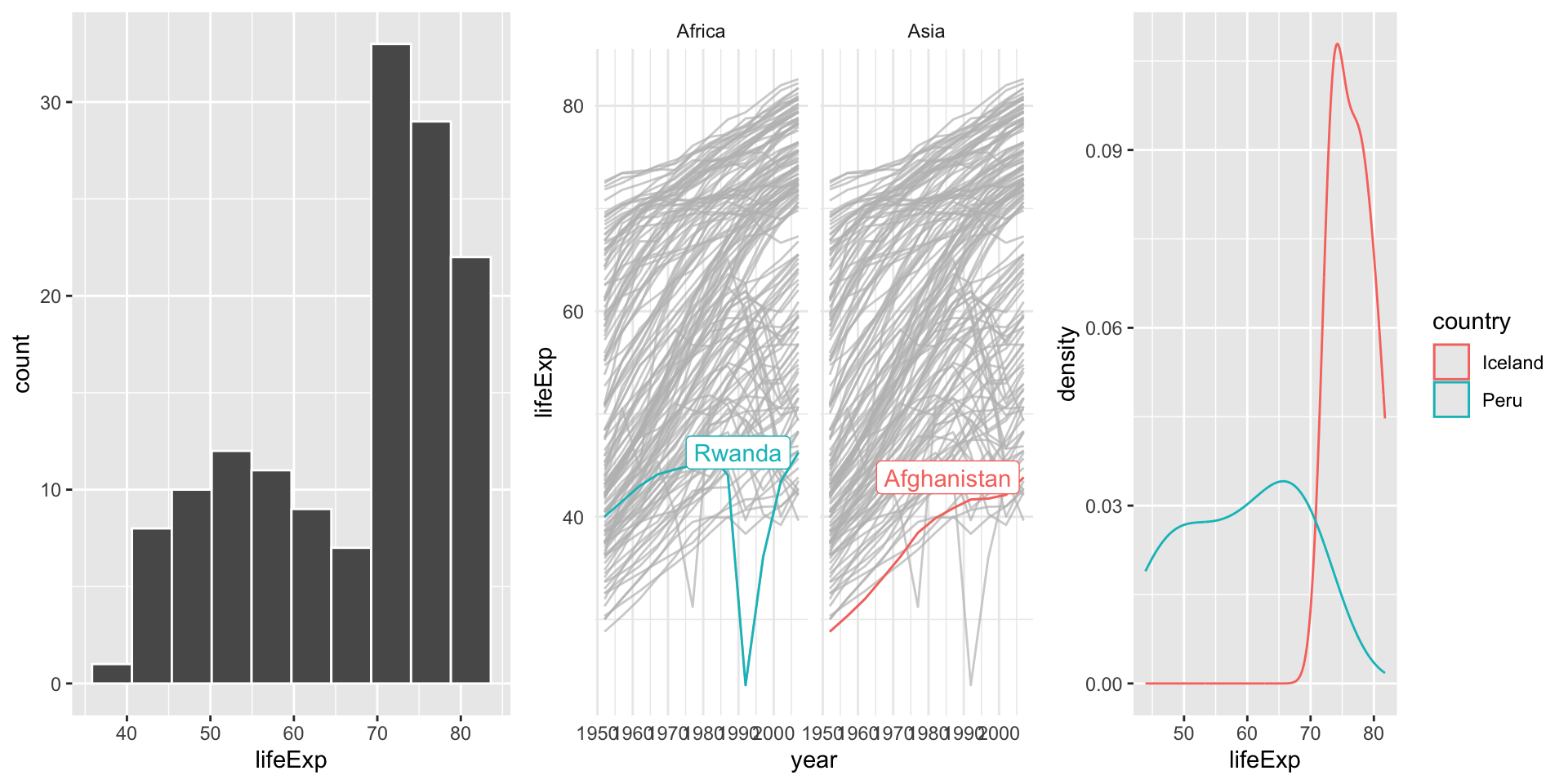
grid and gridExtra examples continued…
Passing plots to grid.arrange() and specifying either the number of rows or columns gives a simple layout.
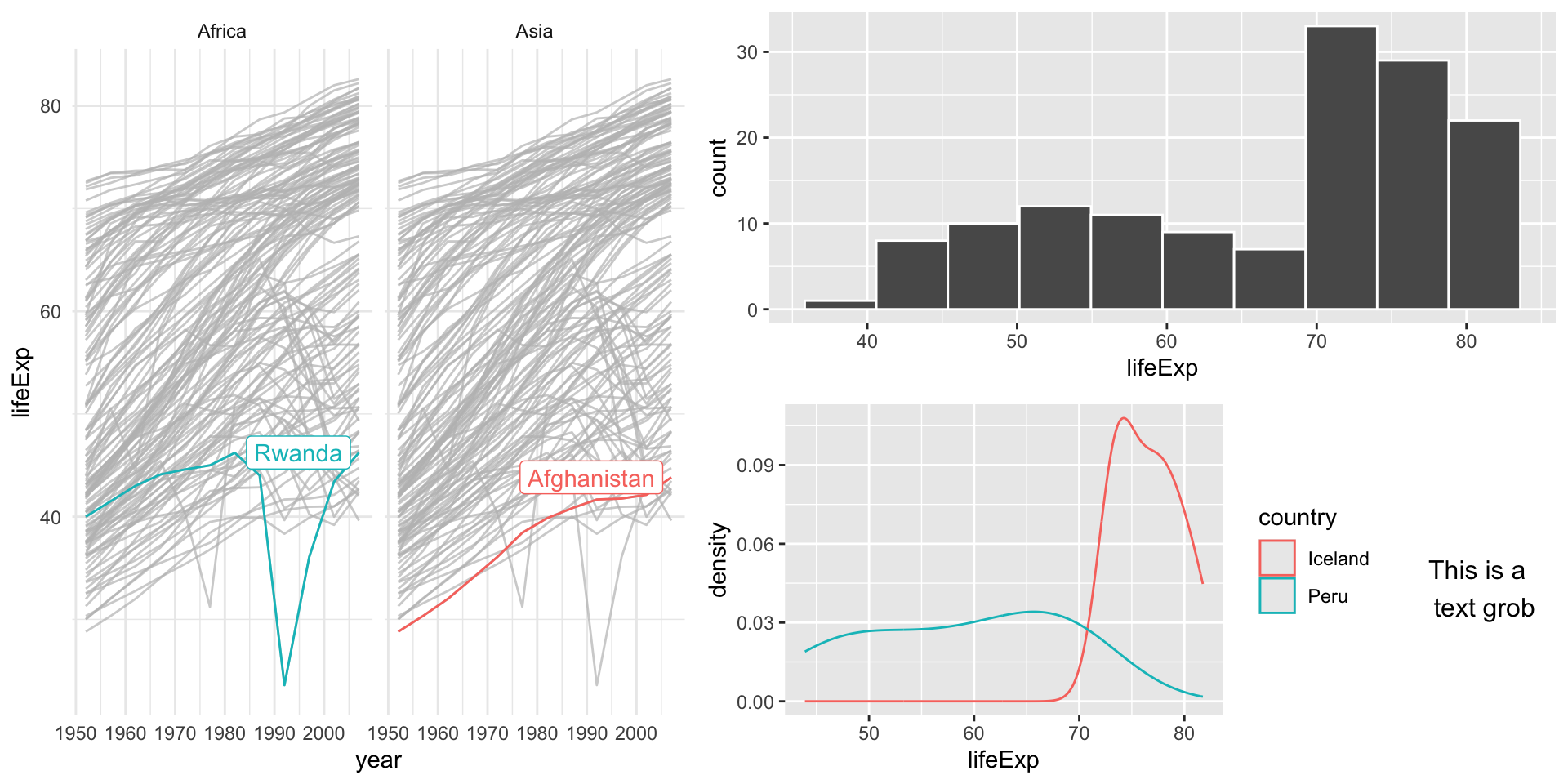
grid and gridExtra examples continued…
Grobs may also be placed in a list and arranged using customized formats using the argument layout_matrix.
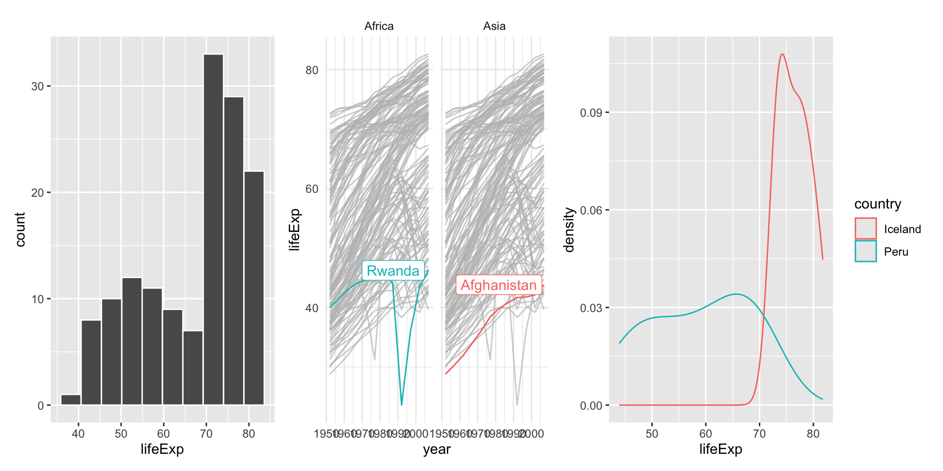
Patchwork
The patchwork package provides a shorthand method to plot multiple ggplot objects together
Patchwork example continued…
To structure plot layouts further use the plot_layout() function
Note that the {} indicate a nested plot
Patchwork example continued…
This package also uses | to indicate plots adjacent to one another and / to indicate vertical stacking
For more examples see: https://gotellilab.github.io/GotelliLabMeetingHacks/NickGotelli/ggplotPatchwork.html
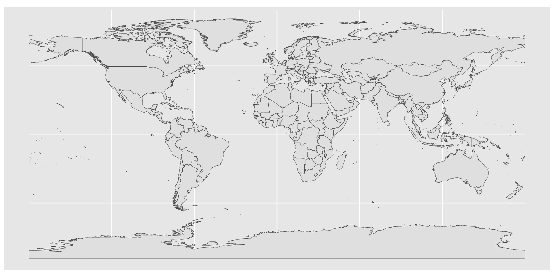
simple map
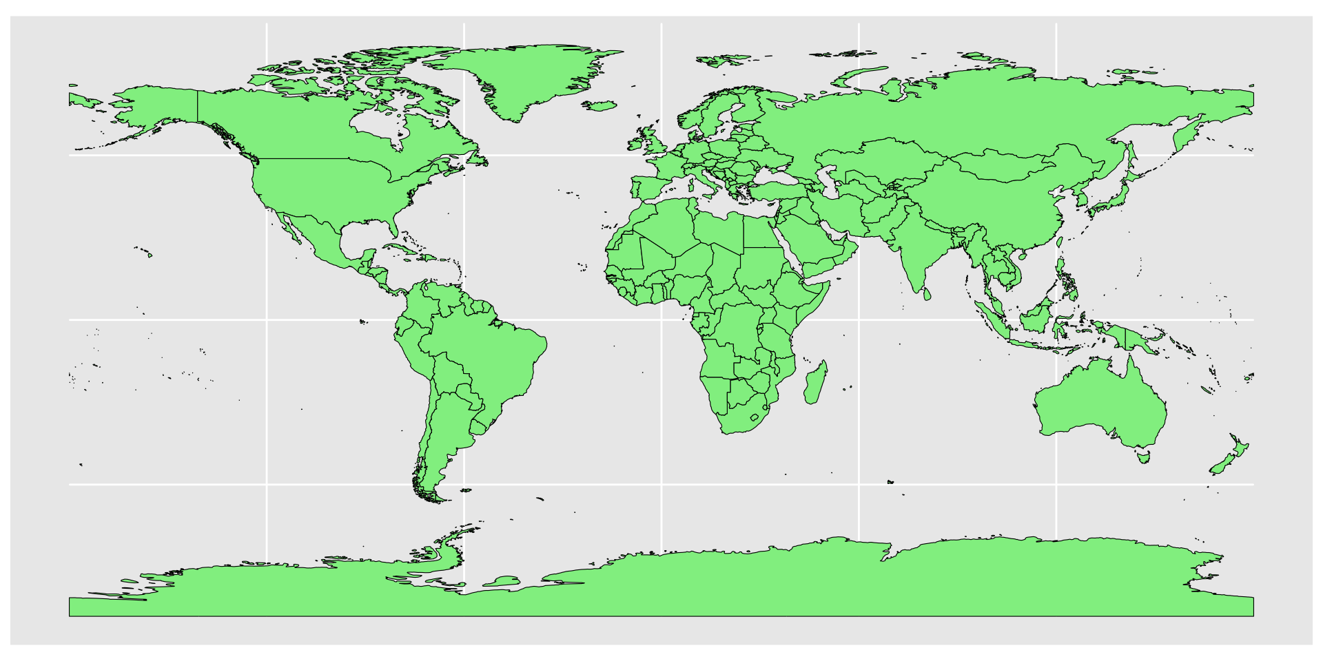
map color
chloropleth maps
plotting a data variable with our geometries
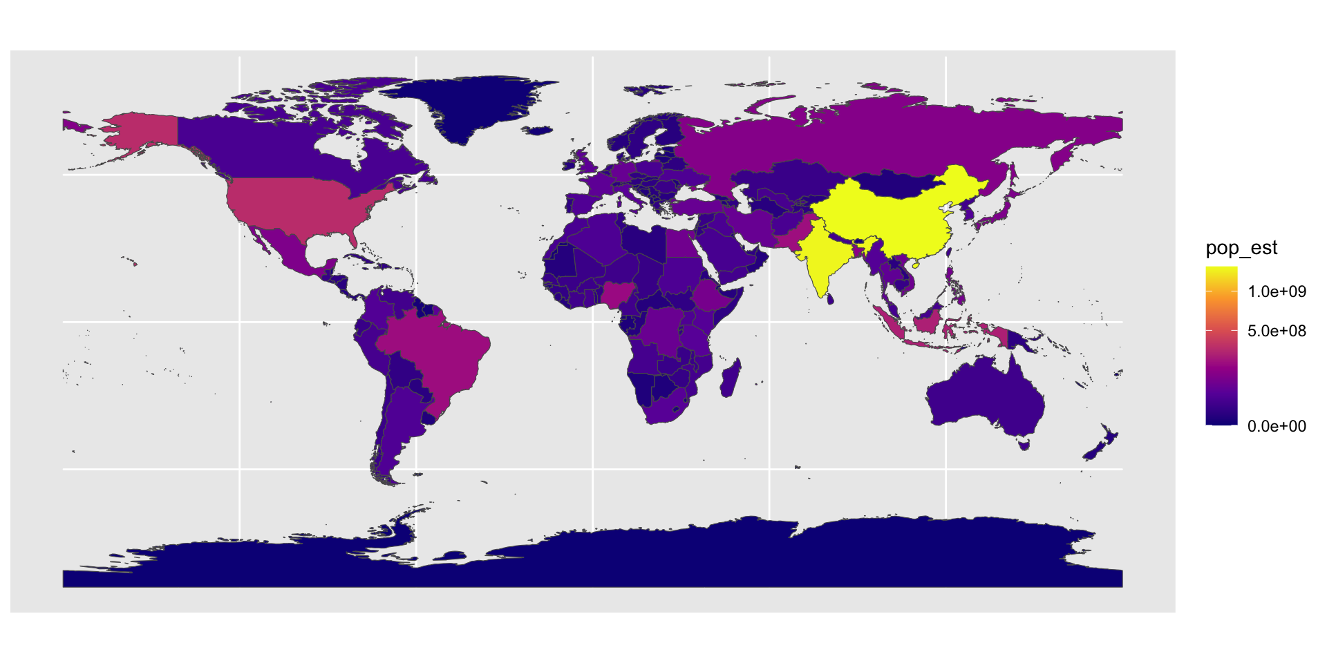
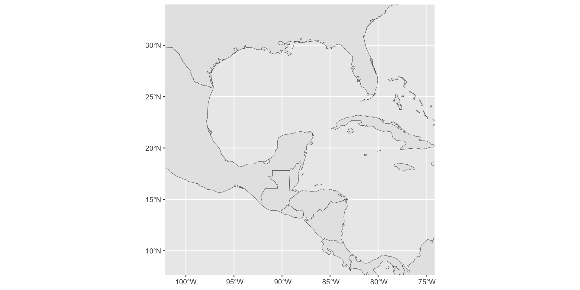
Projection and extent
coord_sf() deals with the coordinate system Used to change the map projections, and the extent. e.g.
census data example
library(tidycensus)
#options(tigris_use_cache = TRUE)

age_data <- get_acs(
  geography = "tract",
  variables = "B19013_001", #"B01002_001",
  state = "MA",
  geometry = TRUE
)
ggplot(age_data, aes(fill = estimate)) +
  geom_sf(color = NA) +
  theme_void() +
  scale_fill_viridis_c(option = "magma") +
  labs(title = "Massachusetts median income",
       subtitle = "2017-2021 ACS",
       fill = "Estimate")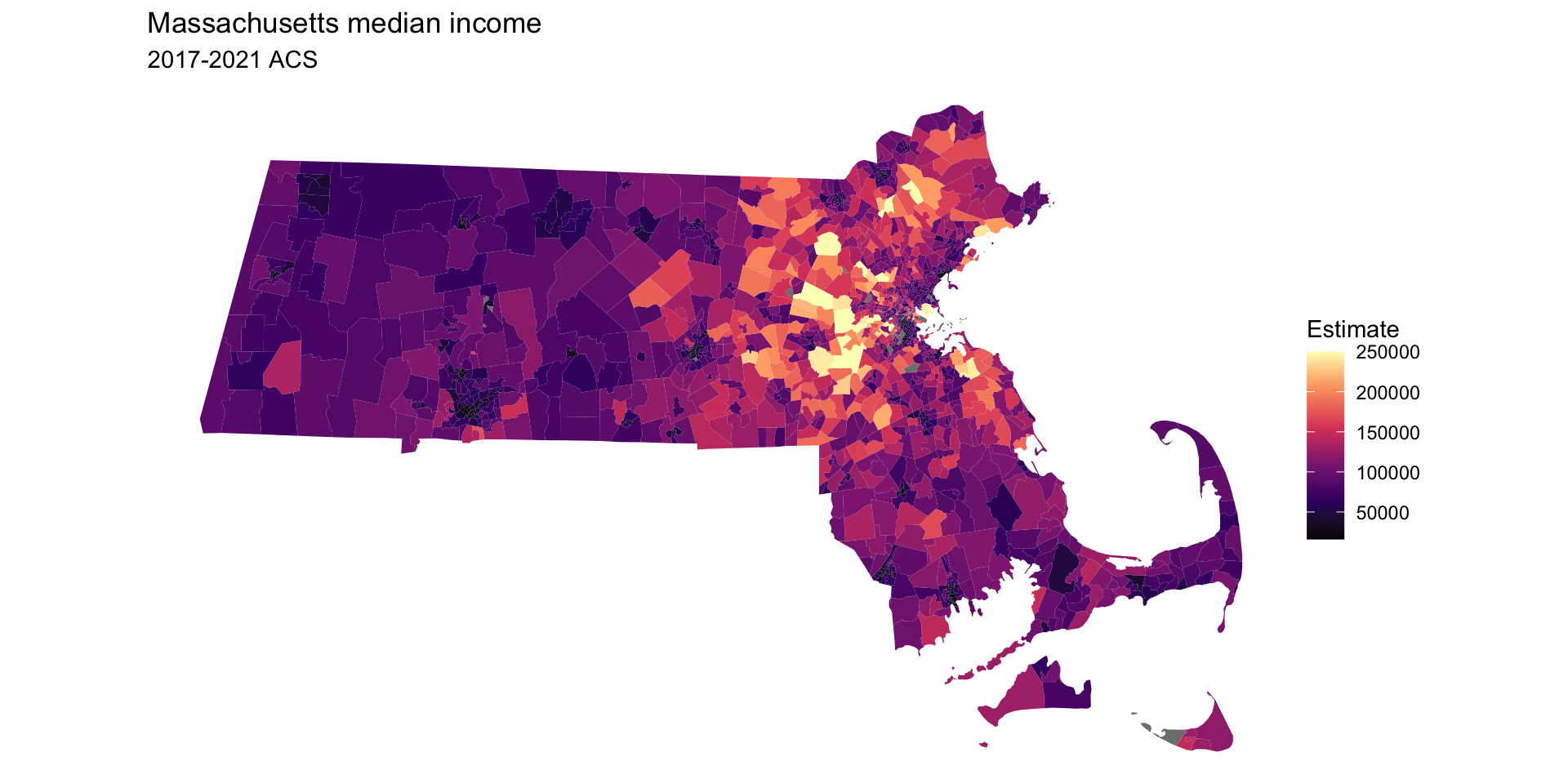
##
  |
  |                                                                      |   0%
  |
  |==                                                                    |   3%
  |
  |====                                                                  |   5%
  |
  |=====                                                                 |   8%
  |
  |=======                                                               |  10%
  |
  |=========                                                             |  13%
  |
  |===========                                                           |  15%
  |
  |=============                                                         |  18%
  |
  |==============                                                        |  21%
  |
  |================                                                      |  23%
  |
  |==================                                                    |  26%
  |
  |====================                                                  |  28%
  |
  |======================                                                |  31%
  |
  |=======================                                               |  33%
  |
  |=========================                                             |  36%
  |
  |=============================                                         |  41%
  |
  |================================                                      |  46%
  |
  |==================================                                    |  49%
  |
  |====================================                                  |  51%
  |
  |=======================================                               |  56%
  |
  |===========================================                           |  61%
  |
  |===============================================                       |  67%
  |
  |==================================================                    |  72%
  |
  |========================================================              |  79%
  |
  |=========================================================             |  82%
  |
  |================================================================      |  92%
  |
  |====================================================================  |  97%
  |
|======================================================================| 100%just for Bristol County
age_data <- get_acs(
  geography = "tract",
  variables = "B19013_001",  #for median age = "B01002_001",
  state = "MA",
  county = "Bristol",
  geometry = TRUE
)

ggplot(age_data, aes(fill = estimate)) +
  geom_sf(color = NA) +
  theme_void() +
  scale_fill_viridis_c(option = "magma") +
  labs(title = "Bristol County median income",
       subtitle = "2017-2021 ACS",
       fill = "Estimate")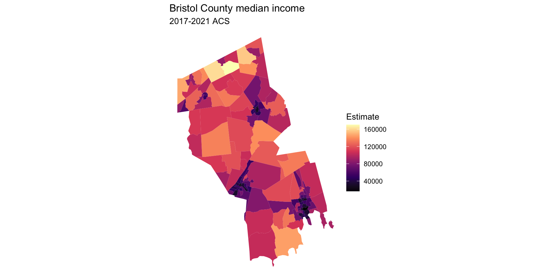
Exercise 2
Use ggplot to create a map of Cape Cod with the following features:
- Longitudes should range from \(-71^{\circ}\text{W}\) to \(-69^{\circ}\text{W}\)
- Latitudes should range from \(41.25^{\circ}\text{N}\) to \(43^{\circ}\text{N}\)
- Label axes
- Color land
- Add points indicating the locations of Woods Hole, Chatham, and Provincetown
- BONUS Change the map projection
For coastline use:
![]()