MAR 536 Lab 6

2023-02-22

Lab schedule

1/18: Introduction to R and R Studio, working with data
1/25: Intro to Visualization
2/01: Probability, linear modeling
2/08: Data wrangling, model summaries
2/15: Simulation, Resampling
2/22: Iteration
3/01: Creating functions, debugging
3/15: Flex: more modeling (brms, glmmTMB)
3/29: Spatial data or tidymodeling

Acknowledgements

Reducing code duplication

Easier to see the intent of your code, eyes are drawn to what’s different, not what stays the same.
Easier to respond to changes, only need to make changes in one place, rather than every place you copied-and-pasted.
Likely to have fewer bugs because each line of code is used in more places.

How? Iteration (today) & Functions (next wk)

Iteration

When you need to do the same thing to multiple inputs: repeating the same operation on different columns, or on different datasets.

Two main paradigms:
1. imperative programming
2. functional programming

Pivot tables & loops

library(palmerpenguins)
for (species in unique(penguins$species)) {
  mean_bodymass <-
      mean(penguins$body_mass_g[penguins$species == species],
           na.rm = TRUE)
  cat(i, mean_bodymass, "\n")
}

with(penguins,tapply(body_mass_g, species, mean, na.rm = TRUE))

aggregate(penguins$body_mass_g, 
          by=list(penguins$species), 
          mean, na.rm = TRUE)

penguins |> 
  group_by(species) |> 
  summarize(mean_bodymass = mean(body_mass_g, na.rm = TRUE))

Looping

Vector operations can do many things and are quick.
But sometimes we need to do more.

Loops in R are of this form:

for (i in set) {
  #do something
}

This is a very flexible structure, try the following:

for (i in seq(from=1,to=5,by=1)) { print(i) }
for (i in 1:100) { print(i) }
for (i in c("1","N","L")) { print(i) }

Looping through species

Imagine we need to calculate the mean flipper and bill lengths for every species in the palmerpenguins data set.

for (species in unique(penguins$species)) {
  mean_flipper_length <-
      mean(penguins$flipper_length_mm[penguins$species == species])   
  mean_bill_length <-
      mean(penguins$bill_length_mm[penguins$species == species])   
  cat(species, mean_flipper_length, mean_bill_length, "\n")
}

NB: We already know better ways to do this using summarize().

Common way to use loops

#define the elements to loop over
species <- sort(unique(penguins$species))

#define how many times to do the loop
nspecies <- length(species)

#create a place to store results
mean_mass <- vector(length=nspecies)

#get loopy
for (isp in 1:nspecies) {
  species.data <- penguins[penguins$species==species[isp], ]
  mean_mass[isp] <- mean(species.data$body_mass_g, na.rm = TRUE)
  print(mean_mass[isp])
  cat("Running species ", isp,"\n")
}

A lot of this code is book-keeping rather than the thing we want to do.

`purrr`

for loops are simple, but they require lots of code that is mostly book-keeping.

Attention is then on this rather than the action the code is doing.

Functional programming abstracts the book-keeping of the loop to keep attention on the code that matters.

Series of apply functions in base R. (apply, tapply, sapply, lapply)
These all have slightly differences about how they are used.

purrr package is the tidyverse solution to the apply functions.

Basics of `purrr`

The map function is the workhorse of purrr.
e.g.

shades <- colors()[1:5]
for (i in seq_along(shades)) { 
  print(shades[i])  
}
## [1] "white"
## [1] "aliceblue"
## [1] "antiquewhite"
## [1] "antiquewhite1"
## [1] "antiquewhite2"

a <-  map(shades, print)
## [1] "white"
## [1] "aliceblue"
## [1] "antiquewhite"
## [1] "antiquewhite1"
## [1] "antiquewhite2"

`map`

Basic syntax:

map("Lists to apply function to",  
    "Function to apply across lists",
    "Additional parameters")

map by default returns a list. However we can specify the type of output:

map_dbl returns real numbers
map_lgl returns logicals
map_chr returns characters
map_int returns integers
map_df returns a dataframe

cheatsheat: github.com/rstudio/cheatsheets/blob/master/purrr.pdf

Shortcuts

models <- penguins %>% 
  split(.$species) %>% 
  map(function(df) lm(body_mass_g ~ flipper_length_mm, data = df))

The syntax for creating an anonymous function in R is quite verbose so purrr provides a convenient shortcut: a one-sided formula.

models <- penguins %>%
  split(.$species) %>% 
  map(~lm(body_mass_g ~ flipper_length_mm, data = .))
  #The 1st ~ is shorthand for a function
  #The '.' shows where the stuff passed to map gets used.

Shortcuts 2

Extracting summary statistics

models |>
  map(summary) |> 
  map_dbl(pluck, "r.squared")

models |>
  map(summary) |> #run 'summary() for each model
  map_dbl(~.$r.squared) # find the R-squared

Extracting named components is a common operation, so can use a string instead.

models |>
  map(summary) |> #run 'summary() for each model
  map_dbl("r.squared") #find the R-squared

Exercise 1

Write code that uses one of the map functions to:

Compute the mean of every numeric column in palmerpenguins::penguins.

Determine the type of each column in nycflights13::flights.

Compute the number of unique values in each column of palmerpenguins::penguins.

05:00

Extending to multiple input lists

map2 allows you to map over two sets of inputs.

map2(list1, list2, ~function(.x,.y), ...)

e.g. generate 3 sets of 5 normal random variables, with the means & standard deviations different in each set.

mu <- list(5, 10, -3)
sigma <- list(1, 5, 10)
map2(mu, sigma, rnorm, n = 5) |> str()
## List of 3
##  $ : num [1:5] 4.78 5.28 5.6 4.46 4.92
##  $ : num [1:5] 9.83 4.23 16.61 6.71 16.3
##  $ : num [1:5] 2.438 4.681 -3.453 -16.228 0.252

More than 2 inputs, use `pmap`

e.g. same problem as previous, but now n varies in each set.

n <- list(1, 3, 5)
mu <- list(5, 10, -3)
sigma <- list(1, 5, 10)

args1 <- list(mean = mu, sd = sigma, n = n)
args1 |>
  pmap(rnorm) |>
  str()
## List of 3
##  $ : num 7.46
##  $ : num [1:3] 14.17 9.36 4.04
##  $ : num [1:5] -15.98 -15.89 -17.65 5.46 3.53

Safest to use named arguments with pmap, as it will do positional matching if not.

Debugging using `safely`

Handling errors can be tricky to diagnose with map.
It’s not as obvious when/where things break.

Can use safely(). e.g.

safe_log <- safely(log, otherwise = NA_real_) 
#safe_log return a NA if log() returns error, plus error msg.  
list("a", 10, 100) |>
  map(safe_log) |>  #<<
  transpose() |>
  simplify_all()
## $result
## [1]       NA 2.302585 4.605170
## 
## $error
## $error[[1]]
## <simpleError in .Primitive("log")(x, base): non-numeric argument to mathematical function>
## 
## $error[[2]]
## NULL
## 
## $error[[3]]
## NULL

Exercise 2

Create a data frame of samples from the palmerpenguins::penguins dataset, that contains 3 Adelies, 6 Gentoos, and 4 Chinstraps.
(your new data frame will have 13 rows, with 3, 6, and 4 of the three species) (hint: use a nested dataframe, map2(), and slice_sample())
We have data from several years of crab surveys. The data for each year is contained in separate “.csv” files.

We would like to read these data into R, and combine them into a single data frame so we can inspect and plot them.

Write code to read these data into R, and combine them into a single dataframe.

b-d. Then produce 3 plots (of your choice) summarizing the full dataset. Include “b”, “c”, and “d” in the title of your plots.

For hints see next slide.

Hints for exercise 2:

you can use the following to get an object containing a list of files in a folder
::: {.cell}

data_path = "../data/crabs"  # directory where the files are located
files <- dir(path = data_path, pattern = "*.csv",
             full.names = TRUE) # names of files ending in ".csv"
files
##  [1] "../data/crabs/CRABS_2001.csv" "../data/crabs/CRABS_2002.csv"
##  [3] "../data/crabs/CRABS_2003.csv" "../data/crabs/CRABS_2004.csv"
##  [5] "../data/crabs/CRABS_2005.csv" "../data/crabs/CRABS_2006.csv"
##  [7] "../data/crabs/CRABS_2007.csv" "../data/crabs/CRABS_2008.csv"
##  [9] "../data/crabs/CRABS_2009.csv" "../data/crabs/CRABS_2010.csv"
## [11] "../data/crabs/CRABS_2011.csv" "../data/crabs/CRABS_2012.csv"
## [13] "../data/crabs/CRABS_2013.csv" "../data/crabs/CRABS_2014.csv"
## [15] "../data/crabs/CRABS_2015.csv" "../data/crabs/CRABS_2016.csv"
## [17] "../data/crabs/CRABS_2017.csv" "../data/crabs/CRABS_2018.csv"
## [19] "../data/crabs/CRABS_2019.csv"

::: - look at the help for ‘dir’ for additional functionality

Steller sea lion pups revisited

We have data on Steller sea lion pup counts over time at a bunch of rookeries in Alaska.

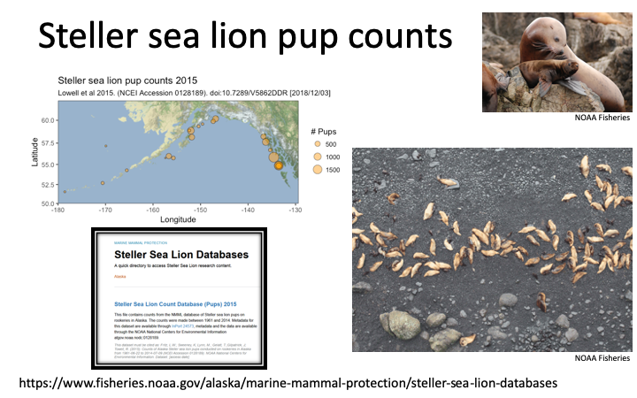
The number of data points for each rookery is not the same.

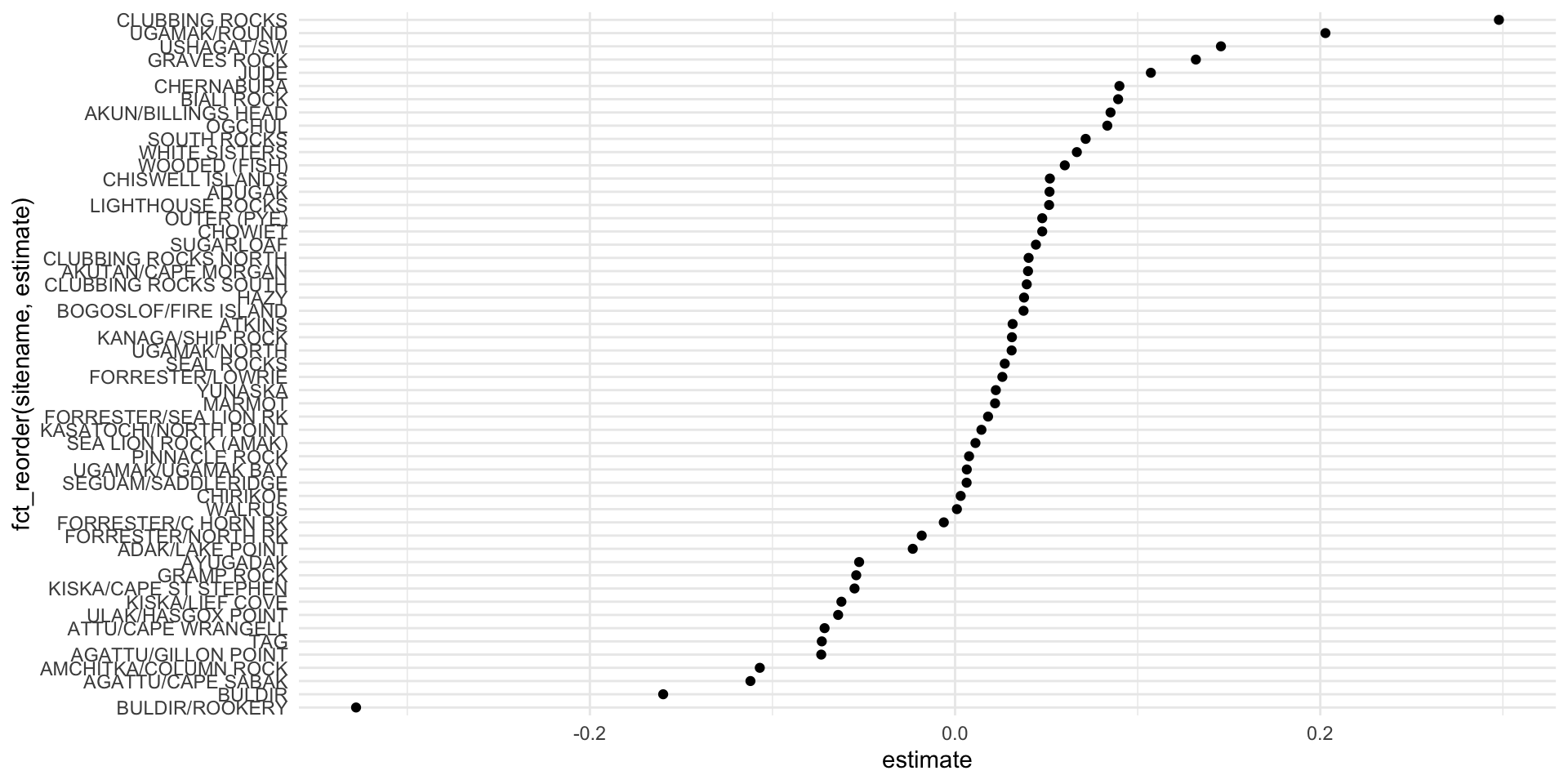
We want to investigate the annual trend in counts for each rookery.
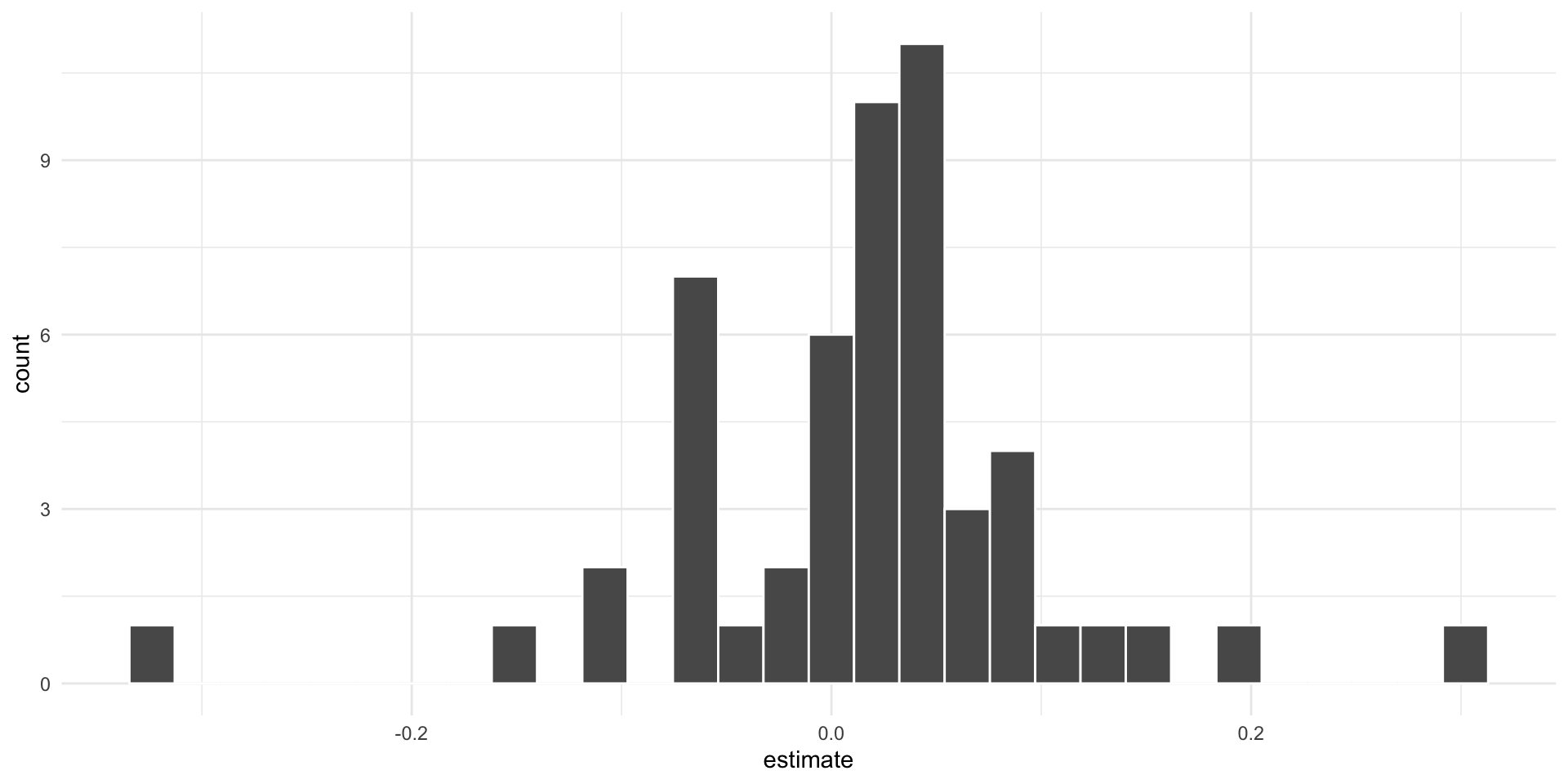
We want to plot the slopes of the regressions using a histogram.
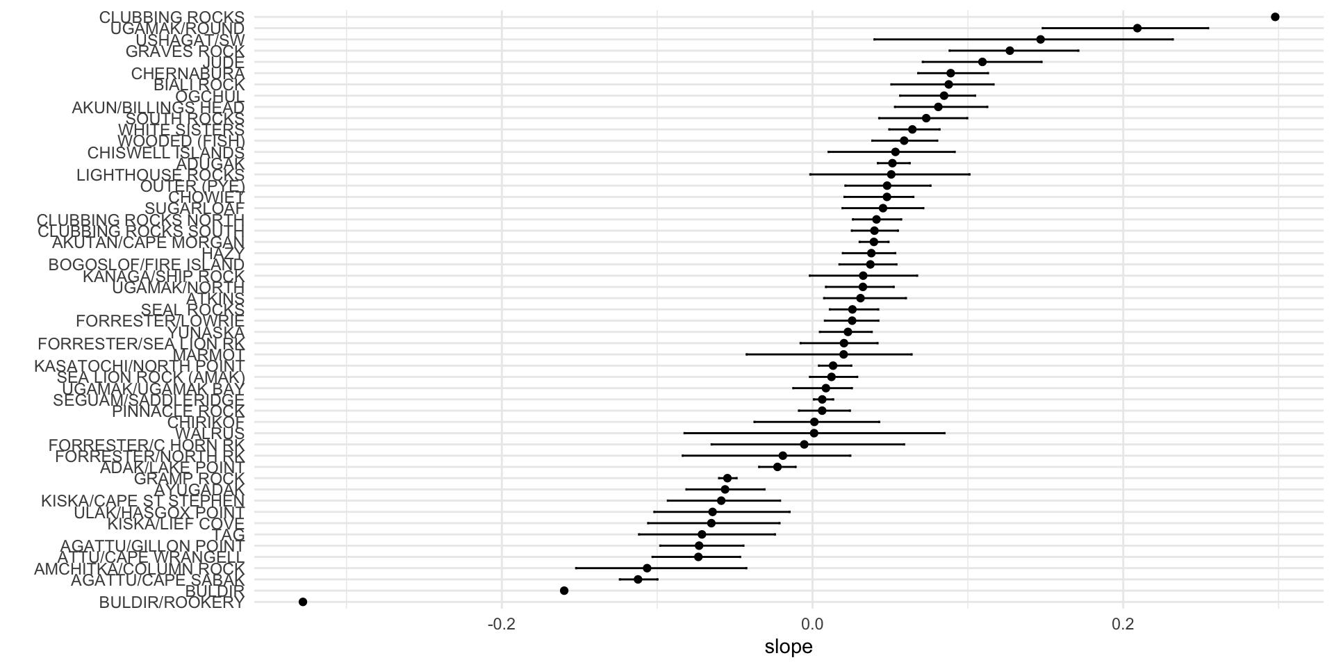
We want to obtain confidence intervals of the slope estimates using bootstrapping.

ssl <- read_csv("../data/SSLpupcounts.csv")
slice(ssl,1:3)
## # A tibble: 3 × 43
##   sitename `1961` `1965` `1967` `1968` `1971` `1973` `1975` `1976` `1978` `1979`
##   <chr>     <dbl>  <dbl>  <dbl>  <dbl>  <dbl>  <dbl>  <dbl>  <dbl>  <dbl>  <dbl>
## 1 ADAK/LA…     NA     NA     NA     NA     NA     NA     NA     NA     NA     20
## 2 ADUGAK       NA     NA     NA     NA     NA     NA     NA     NA     NA     NA
## 3 AGATTU       NA     NA     NA     NA     NA     NA     NA     NA     NA    183
## # … with 32 more variables: `1981` <dbl>, `1982` <dbl>, `1984` <dbl>,
## #   `1985` <dbl>, `1986` <dbl>, `1987` <dbl>, `1988` <dbl>, `1989` <dbl>,
## #   `1990` <dbl>, `1991` <dbl>, `1992` <dbl>, `1993` <dbl>, `1994` <dbl>,
## #   `1995` <dbl>, `1996` <dbl>, `1997` <dbl>, `1998` <dbl>, `2000` <dbl>,
## #   `2001` <dbl>, `2002` <dbl>, `2003` <dbl>, `2004` <dbl>, `2005` <dbl>,
## #   `2007` <dbl>, `2008` <dbl>, `2009` <dbl>, `2010` <dbl>, `2011` <dbl>,
## #   `2012` <dbl>, `2013` <dbl>, `2014` <dbl>, `2015` <dbl>
ssl_long <- ssl |> 
  pivot_longer(names_to = "year",
               values_to = "count",
               -sitename) |> 
  drop_na() |> 
  mutate(year = as.numeric(year)) |> 
  filter(year >= 2000,
         count > 0) |>
  mutate(log_count = log(count),
         year2 = year-2000) |> 
  I()

ssl_models <- ssl_long |>
  group_by(sitename) |> 
  nest() |> 
  mutate(model = map(data, ~lm(log_count ~ year2, data = .))) |> 
  mutate(results = map(model, tidy))
ssl_models
## # A tibble: 53 × 4
## # Groups:   sitename [53]
##    sitename             data              model  results         
##    <chr>                <list>            <list> <list>          
##  1 ADAK/LAKE POINT      <tibble [7 × 4]>  <lm>   <tibble [2 × 5]>
##  2 ADUGAK               <tibble [8 × 4]>  <lm>   <tibble [2 × 5]>
##  3 AGATTU/CAPE SABAK    <tibble [10 × 4]> <lm>   <tibble [2 × 5]>
##  4 AGATTU/GILLON POINT  <tibble [8 × 4]>  <lm>   <tibble [2 × 5]>
##  5 AKUN/BILLINGS HEAD   <tibble [7 × 4]>  <lm>   <tibble [2 × 5]>
##  6 AKUTAN/CAPE MORGAN   <tibble [8 × 4]>  <lm>   <tibble [2 × 5]>
##  7 AMCHITKA/COLUMN ROCK <tibble [5 × 4]>  <lm>   <tibble [2 × 5]>
##  8 ATKINS               <tibble [9 × 4]>  <lm>   <tibble [2 × 5]>
##  9 ATTU/CAPE WRANGELL   <tibble [8 × 4]>  <lm>   <tibble [2 × 5]>
## 10 AYUGADAK             <tibble [7 × 4]>  <lm>   <tibble [2 × 5]>
## # … with 43 more rows

ssl_slopes <- ssl_models |> 
  select(sitename, results) |>
  unnest() |>
  filter(term == "year2")
ssl_slopes
## # A tibble: 53 × 6
## # Groups:   sitename [53]
##    sitename             term  estimate std.error statistic    p.value
##    <chr>                <chr>    <dbl>     <dbl>     <dbl>      <dbl>
##  1 ADAK/LAKE POINT      year2  -0.0232   0.00738     -3.14 0.0256    
##  2 ADUGAK               year2   0.0517   0.00633      8.17 0.000181  
##  3 AGATTU/CAPE SABAK    year2  -0.112    0.00877    -12.8  0.00000133
##  4 AGATTU/GILLON POINT  year2  -0.0733   0.0168      -4.35 0.00482   
##  5 AKUN/BILLINGS HEAD   year2   0.0851   0.0190       4.49 0.00648   
##  6 AKUTAN/CAPE MORGAN   year2   0.0399   0.00602      6.63 0.000566  
##  7 AMCHITKA/COLUMN ROCK year2  -0.107    0.0333      -3.21 0.0488    
##  8 ATKINS               year2   0.0315   0.0207       1.52 0.172     
##  9 ATTU/CAPE WRANGELL   year2  -0.0715   0.0176      -4.06 0.00667   
## 10 AYUGADAK             year2  -0.0525   0.0163      -3.22 0.0234    
## # … with 43 more rows

Plot
Code

plot1 <- ggplot(ssl_slopes) +
  aes(x = estimate) +
  geom_histogram(col="white") +
  theme_minimal()
plot1

Plot
Code

plot2 <- ggplot(ssl_slopes) +
  aes(x = fct_reorder(sitename, estimate), y= estimate) +
  geom_point() +
  coord_flip() +
  theme_minimal()
plot2

residual bootstrapping

resample residuals from the original models to obtain bootstrapped confidence intervals of the slopes.

nboot <- 100
# first extract a table of fitted values and residuals using augment
ssl_boot <- ssl_models |>
  mutate(tbl = map(model, augment)) |> 
  select(sitename, tbl)
ssl_boot
## # A tibble: 53 × 2
## # Groups:   sitename [53]
##    sitename             tbl              
##    <chr>                <list>           
##  1 ADAK/LAKE POINT      <tibble [7 × 8]> 
##  2 ADUGAK               <tibble [8 × 8]> 
##  3 AGATTU/CAPE SABAK    <tibble [10 × 8]>
##  4 AGATTU/GILLON POINT  <tibble [8 × 8]> 
##  5 AKUN/BILLINGS HEAD   <tibble [7 × 8]> 
##  6 AKUTAN/CAPE MORGAN   <tibble [8 × 8]> 
##  7 AMCHITKA/COLUMN ROCK <tibble [5 × 8]> 
##  8 ATKINS               <tibble [9 × 8]> 
##  9 ATTU/CAPE WRANGELL   <tibble [8 × 8]> 
## 10 AYUGADAK             <tibble [7 × 8]> 
## # … with 43 more rows

residual bootstrapping

nboot <- 100
# first extract a table of fitted values and residuals using augment
ssl_boot <- ssl_models |>
  mutate(tbl = map(model, augment)) |> 
  select(sitename, tbl)|> 
  unnest(cols=c(tbl)) |> 
  janitor::clean_names() |> 
  ungroup() |>
  I()
ssl_boot
## # A tibble: 372 × 9
##    sitename       log_count year2 fitted    resid   hat  sigma  cooksd std_resid
##    <chr>              <dbl> <dbl>  <dbl>    <dbl> <dbl>  <dbl>   <dbl>     <dbl>
##  1 ADAK/LAKE POI…      5.89     2   5.90 -0.00375 0.452 0.0868 0.00176   -0.0653
##  2 ADAK/LAKE POI…      5.86     4   5.85  0.00614 0.277 0.0868 0.00166    0.0929
##  3 ADAK/LAKE POI…      5.74     5   5.83 -0.0888  0.216 0.0709 0.231     -1.29  
##  4 ADAK/LAKE POI…      5.82     9   5.74  0.0886  0.155 0.0722 0.141      1.24  
##  5 ADAK/LAKE POI…      5.76    10   5.71  0.0509  0.184 0.0821 0.0595     0.726 
##  6 ADAK/LAKE POI…      5.73    11   5.69  0.0454  0.232 0.0829 0.0673     0.667 
##  7 ADAK/LAKE POI…      5.52    14   5.62 -0.0985  0.483 0.0533 1.46      -1.76  
##  8 ADUGAK              5.03     0   4.99  0.0416  0.412 0.0857 0.155      0.666 
##  9 ADUGAK              5.08     2   5.09 -0.0172  0.269 0.0886 0.0112    -0.247 
## 10 ADUGAK              5.12     4   5.20 -0.0778  0.175 0.0804 0.118     -1.05  
## # … with 362 more rows

residual bootstrapping

# we'll do resampling from the residuals for each year within each rookery
# rather than getting complicated with nested lists, we'll use sample_frac() to do the resamples
tosample <- ssl_boot |> 
  select(sitename, resid) |> 
  group_by(sitename)
resamples <-
   map_dfr(seq_len(nboot), ~slice_sample(tosample, prop = 1, replace = TRUE)) |>
   ungroup() |> 
   mutate(replicate = rep(1:nboot, each = nrow(tosample)))
resamples
## # A tibble: 37,200 × 3
##    sitename          resid replicate
##    <chr>             <dbl>     <int>
##  1 ADAK/LAKE POINT  0.0454         1
##  2 ADAK/LAKE POINT  0.0509         1
##  3 ADAK/LAKE POINT  0.0509         1
##  4 ADAK/LAKE POINT  0.0886         1
##  5 ADAK/LAKE POINT  0.0454         1
##  6 ADAK/LAKE POINT  0.0509         1
##  7 ADAK/LAKE POINT -0.0985         1
##  8 ADUGAK          -0.0384         1
##  9 ADUGAK          -0.0193         1
## 10 ADUGAK          -0.0778         1
## # … with 37,190 more rows

resamples contains our bootstraps. Let’s append them to the data frame so we can compute the new data and re-fit the models for each case.

ssl_bootmod <- map_dfr(seq_len(nboot), ~I(ssl_boot)) |>
  select(-resid, -sitename) |> 
  bind_cols(resamples) |> 
  mutate(log_count = fitted + resid) |> 
  group_by(sitename, replicate) |> 
  nest() # now have a data frame with a row for each site & replicate
ssl_bootmod
## # A tibble: 5,300 × 3
## # Groups:   sitename, replicate [5,300]
##    sitename             replicate data             
##    <chr>                    <int> <list>           
##  1 ADAK/LAKE POINT              1 <tibble [7 × 8]> 
##  2 ADUGAK                       1 <tibble [8 × 8]> 
##  3 AGATTU/CAPE SABAK            1 <tibble [10 × 8]>
##  4 AGATTU/GILLON POINT          1 <tibble [8 × 8]> 
##  5 AKUN/BILLINGS HEAD           1 <tibble [7 × 8]> 
##  6 AKUTAN/CAPE MORGAN           1 <tibble [8 × 8]> 
##  7 AMCHITKA/COLUMN ROCK         1 <tibble [5 × 8]> 
##  8 ATKINS                       1 <tibble [9 × 8]> 
##  9 ATTU/CAPE WRANGELL           1 <tibble [8 × 8]> 
## 10 AYUGADAK                     1 <tibble [7 × 8]> 
## # … with 5,290 more rows

ssl_bootmod <- ssl_bootmod |>
  mutate(model = map(data, ~lm(log_count ~ year2, data = .))) |>  #same code as before to run the models
  mutate(coef = map(model, coef)) |> 
  mutate(slope = map_dbl(coef, pluck, 2)) |> 
    ungroup()
ssl_bootmod
## # A tibble: 5,300 × 6
##    sitename             replicate data              model  coef        slope
##    <chr>                    <int> <list>            <list> <list>      <dbl>
##  1 ADAK/LAKE POINT              1 <tibble [7 × 8]>  <lm>   <dbl [2]> -0.0309
##  2 ADUGAK                       1 <tibble [8 × 8]>  <lm>   <dbl [2]>  0.0674
##  3 AGATTU/CAPE SABAK            1 <tibble [10 × 8]> <lm>   <dbl [2]> -0.117 
##  4 AGATTU/GILLON POINT          1 <tibble [8 × 8]>  <lm>   <dbl [2]> -0.107 
##  5 AKUN/BILLINGS HEAD           1 <tibble [7 × 8]>  <lm>   <dbl [2]>  0.0956
##  6 AKUTAN/CAPE MORGAN           1 <tibble [8 × 8]>  <lm>   <dbl [2]>  0.0360
##  7 AMCHITKA/COLUMN ROCK         1 <tibble [5 × 8]>  <lm>   <dbl [2]> -0.0443
##  8 ATKINS                       1 <tibble [9 × 8]>  <lm>   <dbl [2]>  0.0457
##  9 ATTU/CAPE WRANGELL           1 <tibble [8 × 8]>  <lm>   <dbl [2]> -0.0630
## 10 AYUGADAK                     1 <tibble [7 × 8]>  <lm>   <dbl [2]> -0.0833
## # … with 5,290 more rows

ssl_bootslopes <- ssl_bootmod |>
  group_by(sitename) |> #pull out summaries of the distribution for the slope estimates for plotting
  summarize(med = median(slope),
            lower = quantile(slope, 0.025),
            upper = quantile(slope, 0.975)) |> 
  I()
ssl_bootslopes
## # A tibble: 53 × 4
##    sitename                 med    lower   upper
##    <chr>                  <dbl>    <dbl>   <dbl>
##  1 ADAK/LAKE POINT      -0.0226 -0.0344  -0.0108
##  2 ADUGAK                0.0514  0.0420   0.0626
##  3 AGATTU/CAPE SABAK    -0.112  -0.124   -0.0998
##  4 AGATTU/GILLON POINT  -0.0730 -0.0980  -0.0445
##  5 AKUN/BILLINGS HEAD    0.0810  0.0530   0.113 
##  6 AKUTAN/CAPE MORGAN    0.0395  0.0303   0.0490
##  7 AMCHITKA/COLUMN ROCK -0.106  -0.152   -0.0426
##  8 ATKINS                0.0309  0.00741  0.0602
##  9 ATTU/CAPE WRANGELL   -0.0735 -0.103   -0.0466
## 10 AYUGADAK             -0.0563 -0.0812  -0.0309
## # … with 43 more rows

Plot
Code

p1 <- ggplot(ssl_bootslopes) +
  aes(x = fct_reorder(sitename, med), y = med) +
  geom_point() +
  geom_errorbar(aes(ymin=lower, ymax=upper), width= 0.2) + #add the bootstrap confidence interval
  coord_flip() +
  theme_minimal() +
  labs(y = "slope",
       x = "") +
  NULL #})
p1

`accumulate()`

We sometimes like to use the output of one iteration as input to the next. e.g. model population dynamics over time, iterated function is annual population update.

\[N_{t+1} = \lambda N_{t} - h_{t}\]

Can achieve this using accumulate().

pop_update <- function(N, h=0, lambda = 1.05) lambda*N - h
h <- rep(10,10)
initN <- 100
accumulate(h, pop_update, .init = initN, lambda = 1.05)
##  [1] 100.00000  95.00000  89.75000  84.23750  78.44938  72.37184  65.99044
##  [8]  59.28996  52.25446  44.86718  37.11054

accumulate(letters[1:10], paste, sep = " + ")
##  [1] "a"                                    
##  [2] "a + b"                                
##  [3] "a + b + c"                            
##  [4] "a + b + c + d"                        
##  [5] "a + b + c + d + e"                    
##  [6] "a + b + c + d + e + f"                
##  [7] "a + b + c + d + e + f + g"            
##  [8] "a + b + c + d + e + f + g + h"        
##  [9] "a + b + c + d + e + f + g + h + i"    
## [10] "a + b + c + d + e + f + g + h + i + j"

Population projections

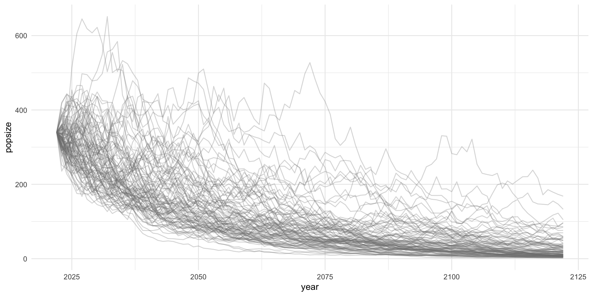
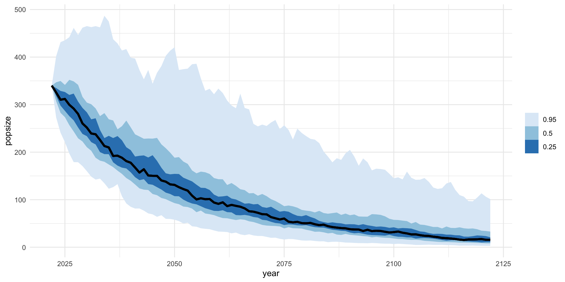
Status for endangered species are often based on a risk evaluation of population projections. We want to project population dynamics forward in time given uncertainty in future dynamics. We want to do this lots of times to quantify the risk of extinction.

Current (2022) estimates of the North Atlantic Right Whale population are 340 individuals. The population has been declining on average around 3% per year since 2011. What is the year in which the probability that the right whale population drops below 100 individuals is at least 50% (P(N<100)>=0.5)?

nsim <- 100
nyr <- 100
initN <- 340
sd_proc <- 0.1
lambda <- 0.97
growth_rates <- map(seq_len(nsim), ~rlnorm(nyr,log(lambda),sd_proc))

# population model
pop_update <- function(N, growth_rate = 1) N*growth_rate

# population projection for each time series of process errors
pop_proj <- tibble(sim = seq_len(nsim)) |>
  mutate(popsize = map(growth_rates,~accumulate(., pop_update, 
                                                .init = initN))) |>
  unnest(cols = c(popsize)) |>
  mutate(year = rep(2022:2122, nsim))
pop_proj
## # A tibble: 10,100 × 3
##      sim popsize  year
##    <int>   <dbl> <int>
##  1     1    340   2022
##  2     1    300.  2023
##  3     1    294.  2024
##  4     1    360.  2025
##  5     1    376.  2026
##  6     1    386.  2027
##  7     1    309.  2028
##  8     1    298.  2029
##  9     1    230.  2030
## 10     1    202.  2031
## # … with 10,090 more rows

Plot
Code

pop_proj |>
  ggplot() +
  aes(x = year,
      y = popsize,
      group = sim) +
  geom_line(alpha = 0.3, col=gray(0.5)) +
  theme_minimal()

Plot
Code

library(ggdist)
pop_proj |>
  group_by(year) |>
  median_qi(popsize, .width = c(.25, .5, .95)) |>
  ggplot() +
  aes(x = year,
      y = popsize,
      ymin = .lower,
      ymax = .upper) +
  geom_lineribbon() +
  scale_fill_brewer() +
  theme_minimal()

below_thresh <- pop_proj |>
  group_by(year) |>
  summarize(prob_100 = mean(popsize<100))
yr_crash <- filter(below_thresh, prob_100 > 0.5) |> slice(1)
yr_crash
## # A tibble: 1 × 2
##    year prob_100
##   <int>    <dbl>
## 1  2059     0.54
below_thresh
## # A tibble: 101 × 2
##     year prob_100
##    <int>    <dbl>
##  1  2022        0
##  2  2023        0
##  3  2024        0
##  4  2025        0
##  5  2026        0
##  6  2027        0
##  7  2028        0
##  8  2029        0
##  9  2030        0
## 10  2031        0
## # … with 91 more rows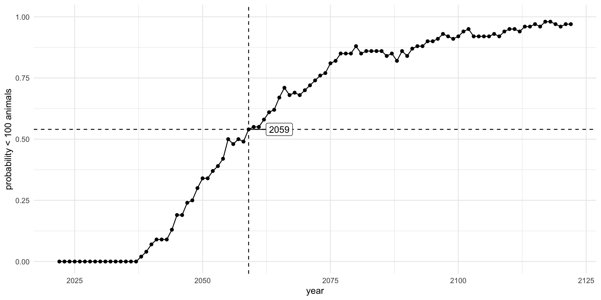

Plot
Code

library(ggrepel)
below_thresh |>
  ggplot() +
  aes(x = year,
      y = prob_100) +
  geom_point() +
  geom_line() +
  labs(x = "year",
       y = "probability < 100 animals") +
  ylim(0,1) +
  theme_minimal() +
  geom_vline(data = yr_crash, aes(xintercept = year), lty = 2) +
  geom_hline(data = yr_crash, aes(yintercept = prob_100), lty = 2) +
  geom_label_repel(data = yr_crash, aes(label = year), nudge_x = 6)

The `while` loop

Occasionally we don’t know how many times to execute the loop.

Can use a while loop, which executes a series of statements for as long as some condition remains true.

The general syntax is:

while (condition) {
  #statements
}

The `while` loop

If there are 7,500 snow leopards in year 2023 and they are declining at 5% per year, in what year will they fall below 500 individuals?

leopard.loop <- function(N, year=2023) {
  while (N>=500) {
    N <- N*0.95
    year <- year+1
  }
  return(year)
}
leopard.loop(N=7500)
[1] 2076

Pro-tip: when you end up in an infinite loop with no stopping point, press <ESC> to stop it running!

Notes on `for` loops

for() loops are used in R code much less often than in compiled languages.

Code that takes a ‘whole object’ view is likely to be both clearer and faster in R.

Other looping facilities include repeat, apply, tapply, lapply, sapply.

The break statement can be used to terminate any loop, possibly abnormally.
This is the only way to terminate repeat loops.

The next statement can be used to discontinue one particular cycle and skip to the “next”.

Improving speed of loops

Looping over very large data sets can sometimes become slow in R. Overcome by:

create storage objects apriori (don’t grow objects).
eliminate certain operations in loops or
avoidg loops over the data-intensive dimension in an object altogether.

the latter can be achieved by performing mainly vector-to-vecor or matrix-to-matrix computations (often > 100x faster than for() or apply() or map()).

Make use of existing speed-optimized R functions (e.g.: rowSums, rowMeans, table) or write your own fast functions.

xdat <- matrix(rnorm(1000000), 100000, 10)
system.time(x_mean <- apply(xdat, 1, mean))
   user  system elapsed 
  1.214   0.029   4.087 
system.time(x_mean <- rowMeans(xdat))
   user  system elapsed 
  0.005   0.001   0.013

Lab Exercise 3/3

data/eukaryotes.tsv contains a NCBI Eukaryotic genome dataset, with basic information about the genomic content of all eukaryotes that were uploaded to the NCBI Genome database.
It contains accession numbers, information about the quality of the genome and stats such a average genome size and GC-content.
Use glimpse() and other data exploration to get familiar with the data. Then use map_* functions to answer the following:

How many different organisms are there in the dataset?
How many different institutes (centers) submitted a genome?
The data seem to be grouped in groups. How many groups are there?
How many sub groups are there?
How many different organisms are there per group?
How many different institutes (centers) submitted a genome per group?
How many sub groups are there per group?

Lab Exercise 3 continued…

We might hypothesisze that “The bigger the size of a genome, the higher the number of proteins”.

Fit a linear model of log10_proteins ~ log10_size_mb for each group.
Extract the R^2 for each model and print these for each group.
Assess the validity of your modeling approach.
Obtain and plot predictions for each group for genome sizes 0.5, 123, and 500 MB.
How do you interpret the results in terms of the original hypothesis?

BONUS use residual bootstrapping to obtain distributions for the predictions made in part 11.

MAR 536 Lab 6

Lab schedule

Acknowledgements

Reducing code duplication

Iteration

Pivot tables & loops

Looping

Looping through species

Common way to use loops

purrr

Basics of purrr

map

Shortcuts

Shortcuts 2

Exercise 1

Extending to multiple input lists

More than 2 inputs, use pmap

Debugging using safely

Exercise 2

Steller sea lion pups revisited

residual bootstrapping

residual bootstrapping

residual bootstrapping

accumulate()

Population projections

The while loop

The while loop

Notes on for loops

Improving speed of loops

Lab Exercise 3/3

Lab Exercise 3 continued…

`purrr`

Basics of `purrr`

`map`

More than 2 inputs, use `pmap`

Debugging using `safely`

`accumulate()`

The `while` loop

The `while` loop

Notes on `for` loops