MAR 536: Lab 4

Gavin Fay

2023-02-08

Lab schedule

1/18: Introduction to R and R Studio, working with data
1/25: Intro to Visualization
2/01: Probability, linear modeling
2/08: Data wrangling, model summaries
2/15: Simulation, Resampling
2/22: Iteration
3/01: Creating functions, debugging
3/15: Flex: more modeling (brms, glmmTMB)
3/29: Spatial data or tidymodeling

Acknowledgements: Mine Çetinkaya-Rundel, Allison Horst

Today

Topics

Poisson GLM
Programming Practices
Data wrangling

setup

library(tidyverse)
library(broom)

#first read in the data (richness already created)
RIKZ <- readRDS("../data/RIKZ.rds")

Generalized linear modeling

All GLMs have the following three characteristics:

A probability distribution describing a generative model for the outcome variable.

A linear model:

\[\eta = \beta_0 + \beta_1 X_1 + \cdots + \beta_k X_k\]

A link function that relates the linear model to the parameter of the outcome distribution.

Generalized linear modeling

Recall from lecture: \[\eta = \beta_1 x_1 + \beta_2 x_2 + \dots + \beta_p x_p\] \[f_Y(y;\mu,\varphi) = \exp\left[\frac{A}{\varphi}{y\lambda(\mu)-\gamma(\lambda(\mu))}+\tau(y,\varphi)\right]\] \[\mu = m(\eta) \text{, } \eta = m^{-1}(\mu)=l(\mu)\]

The combination of a response distribution, a link function and other information needed to carry out the modeling exercise is called the family of the generalized linear model.

The `glm()` function

The R function to fit a generalized linear model is glm() which uses the form:
fitted.model <- glm(formula, family=family.generator, data=data.frame)

Only new piece is the call to ‘family.generator’
Although complex, its use is fairly simple.
Where there is a choice of link, link can be supplied with the family name as a parameter.

Simple (inefficient) use: The following are equivalent.

RIKZ_lm1 <- lm(Richness ~ NAP, data = RIKZ)
RIKZ_glm1 <- glm(Richness ~ NAP, family = gaussian, 
                 data = RIKZ)

Most of the extraction functions that can be applied to lm() can also be used with glm().

The `glm()` function

tidy(RIKZ_lm1)
# A tibble: 2 × 5
  term        estimate std.error statistic  p.value
  <chr>          <dbl>     <dbl>     <dbl>    <dbl>
1 (Intercept)     6.69     0.658     10.2  5.25e-13
2 NAP            -2.87     0.631     -4.55 4.42e- 5
tidy(RIKZ_glm1)
# A tibble: 2 × 5
  term        estimate std.error statistic  p.value
  <chr>          <dbl>     <dbl>     <dbl>    <dbl>
1 (Intercept)     6.69     0.658     10.2  5.25e-13
2 NAP            -2.87     0.631     -4.55 4.42e- 5

Poisson regression

\[P(X=x) = \frac{e^{-\mu} \mu^x}{x!} \text{, } \mu_i = e^{\alpha+\beta_1 x_{1,i} + \dots + \beta_j x_{j,i}}\]

RIKZ example

#fit the poisson regression model
RIKZ_poisson <- glm(Richness ~ NAP, data = RIKZ, 
                    family = poisson)

Note that the default link for the poisson is log so we don’t have to specify here (see ?family).

`summary(RIKZ_poisson)`


Call:
glm(formula = Richness ~ NAP, family = poisson, data = RIKZ)

Deviance Residuals: 
    Min       1Q   Median       3Q      Max  
-2.2029  -1.2432  -0.9199   0.3943   4.3256  

Coefficients:
            Estimate Std. Error z value Pr(>|z|)    
(Intercept)  1.79100    0.06329  28.297  < 2e-16 ***
NAP         -0.55597    0.07163  -7.762 8.39e-15 ***
---
Signif. codes:  0 '***' 0.001 '**' 0.01 '*' 0.05 '.' 0.1 ' ' 1

(Dispersion parameter for poisson family taken to be 1)

    Null deviance: 179.75  on 44  degrees of freedom
Residual deviance: 113.18  on 43  degrees of freedom
AIC: 259.18

Number of Fisher Scoring iterations: 5

`broom::augment()`

As with lm(), the augment() function can be used to obtain the predictions from a fitted model object, and for a new data frame.

newobject <- augment(oldobject, newdata, 
                     type.predict = c("link","response","terms"),
                     se_fit = TRUE)

Note: default for type.predict is on the scale of the linear predictors. Set to "response" to obtain predictions on the scale of the response variable.

augment(RIKZ_poisson, se_fit = TRUE)

# A tibble: 45 × 9
   Richness    NAP .fitted .se.fit .resid .std.resid   .hat .sigma .cooksd
      <dbl>  <dbl>   <dbl>   <dbl>  <dbl>      <dbl>  <dbl>  <dbl>   <dbl>
 1       11  0.045    1.77  0.0639  1.90       1.92  0.0239   1.61 0.0569 
 2       10 -1.04     2.37  0.0896 -0.206     -0.215 0.0856   1.64 0.00213
 3       13 -1.34     2.53  0.106   0.112      0.121 0.142    1.64 0.00122
 4       11  0.616    1.45  0.0827  2.72       2.76  0.0291   1.59 0.165  
 5       10 -0.684    2.17  0.0737  0.406      0.416 0.0476   1.64 0.00453
 6        8  1.19     1.13  0.114   2.32       2.37  0.0401   1.60 0.170  
 7        9  0.82     1.34  0.0929  2.26       2.30  0.0328   1.60 0.125  
 8        8  0.635    1.44  0.0836  1.64       1.66  0.0294   1.62 0.0532 
 9       19  0.061    1.76  0.0641  4.33       4.38  0.0238   1.50 0.376  
10       17 -1.33     2.53  0.106   1.18       1.27  0.141    1.63 0.148  
# … with 35 more rows

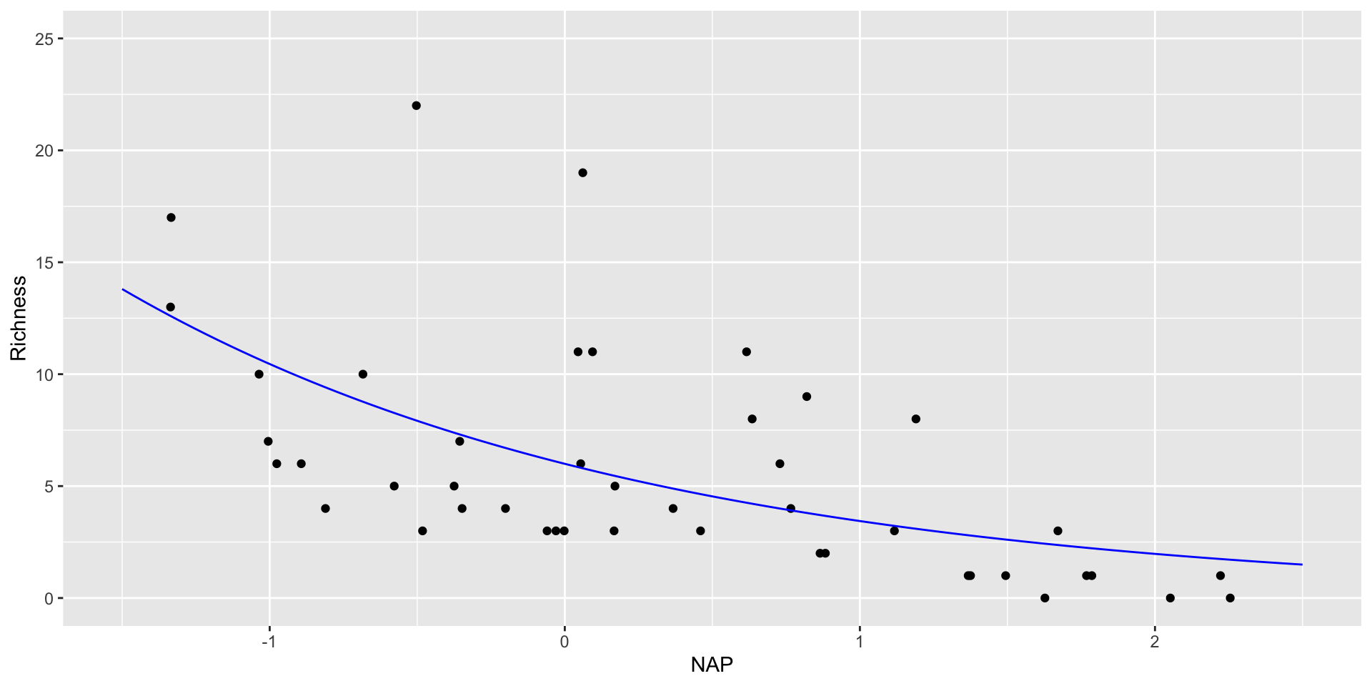
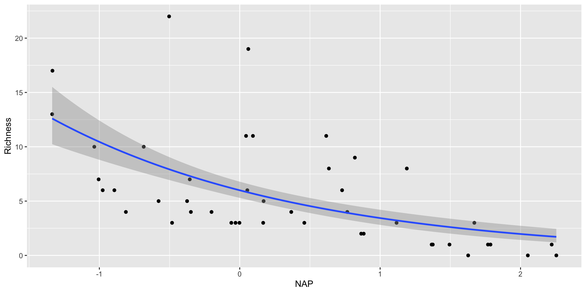
Observed and fitted values for Poisson RIKZ

#create new values for beach height
new_data <- tibble(NAP = seq(-1.5,2.5,length.out=100))
#predict values for response based on new salinity
RIKZ_pois_pred <- augment(RIKZ_poisson,
                    newdata = new_data, 
                    type.predict = "response",
                    se_fit = "TRUE")
RIKZ_pois_pred
# A tibble: 100 × 3
     NAP .fitted .se.fit
   <dbl>   <dbl>   <dbl>
 1 -1.5     13.8    1.60
 2 -1.46    13.5    1.53
 3 -1.42    13.2    1.46
 4 -1.38    12.9    1.40
 5 -1.34    12.6    1.34
 6 -1.30    12.3    1.28
 7 -1.26    12.1    1.23
 8 -1.22    11.8    1.17
 9 -1.18    11.5    1.12
10 -1.14    11.3    1.07
# … with 90 more rows

ggplot(RIKZ, aes(x=NAP, y= Richness)) +
         geom_point() +
         geom_line(data = RIKZ_pois_pred,
                   aes(x=NAP, y = .fitted),
                   col = "blue") +
         labs(y = "Richness", x = "NAP") +
         ylim(0,25) + xlim(-1.5,2.5)

fitting the GLM in the ggplot call

ggplot(RIKZ,aes(NAP,Richness)) +
  geom_point() +
  geom_smooth(method = "glm", 
    method.args = list(family = poisson), se = TRUE)

Lab Exercise 1/4: RIKZ Poisson GLMs

Fit a poisson model to RIKZ species richness that includes NAP, and exposure and week as categorical variables (factor).
Extract the model coefficients and their 95% confidence intervals.
Plot the deviance residuals versus the linear predictor.
Compare the results of this model with a model for RIKZ species richness that only included NAP as a covariate using deviance and AIC.
BONUS Show how AIC changes when each linear predictor term is dropped from the model, and show the results of chi-square tests that compare these reduced models to the original model. (hint see the help for ?add1).
BONUS BONUS Fit a model for species richness that also includes salinity, temperature, and grain size, and perform backwards selection using AIC to obtain a ‘best’ model. How do the results compare to the other models? What is the appropriate set of variables to use?

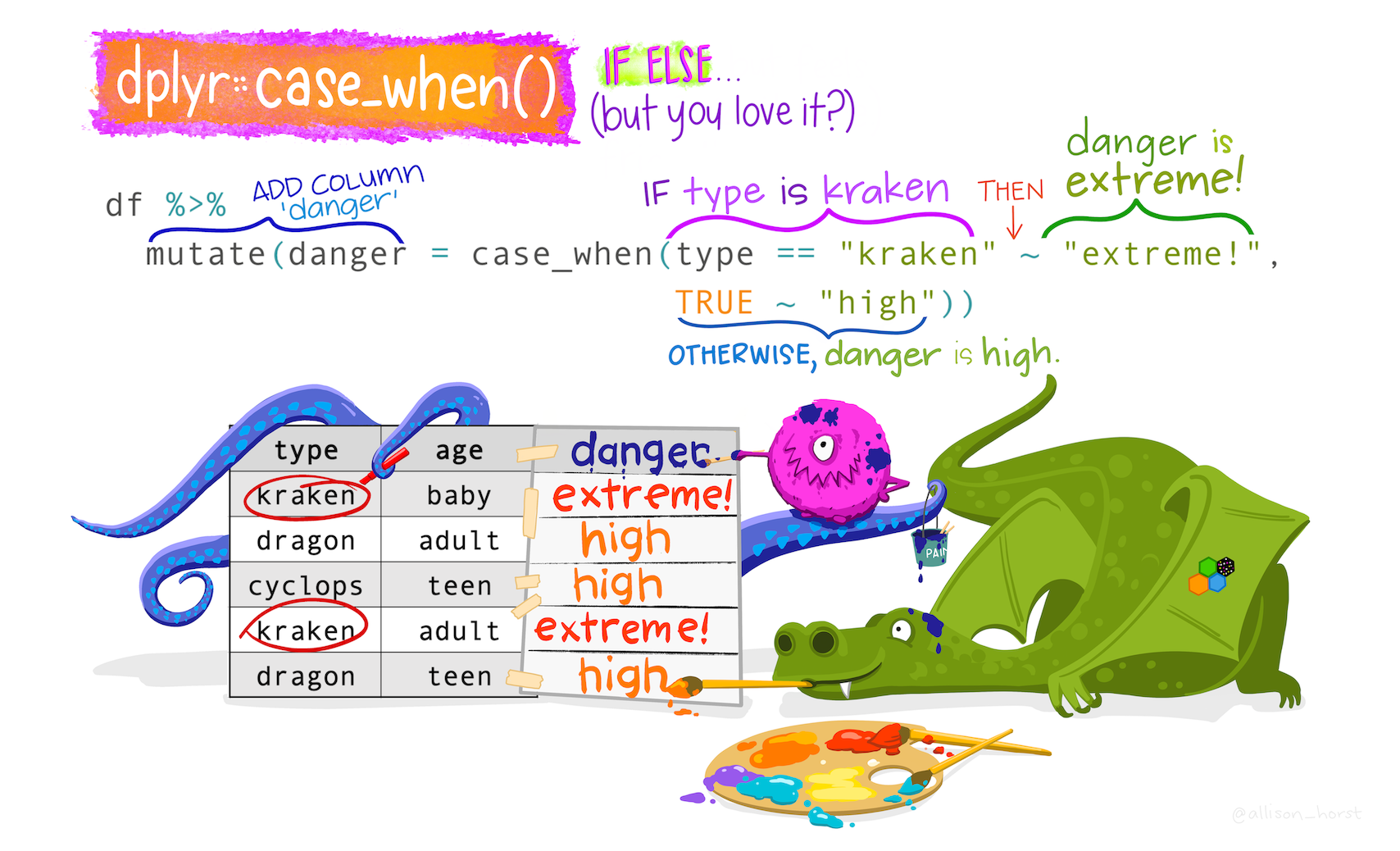
dplyr::case_when()

The case_when() function is like a really friendly if-else statement. When used within mutate(), it allows you to add a new column containing values dependent on your condition(s).

dplyr::case_when()

To penguins, add a new column size_bin that contains:

“large” if body mass is greater than 4500 g
“medium” if body mass is greater than 3000 g, and less than or equal to 4500 g
“small” if body mass is less than or equal to 3000 g

penguins |>
  mutate(size_bin = case_when(
      body_mass_g > 4500 ~ "large",
      body_mass_g > 3000 & body_mass_g <= 4500 ~ "medium",
      body_mass_g <= 3000 ~ "small"
    )
  ) |>
  select(species, island, size_bin, everything())

# A tibble: 344 × 9
   species island    size_bin bill_length_mm bill_depth_mm flipper_length_mm
   <fct>   <fct>     <chr>             <dbl>         <dbl>             <int>
 1 Adelie  Torgersen medium             39.1          18.7               181
 2 Adelie  Torgersen medium             39.5          17.4               186
 3 Adelie  Torgersen medium             40.3          18                 195
 4 Adelie  Torgersen <NA>               NA            NA                  NA
 5 Adelie  Torgersen medium             36.7          19.3               193
 6 Adelie  Torgersen medium             39.3          20.6               190
 7 Adelie  Torgersen medium             38.9          17.8               181
 8 Adelie  Torgersen large              39.2          19.6               195
 9 Adelie  Torgersen medium             34.1          18.1               193
10 Adelie  Torgersen medium             42            20.2               190
# … with 334 more rows, and 3 more variables: body_mass_g <int>, sex <fct>,
#   year <int>

dplyr::case_when()

Starting with penguins:

Limit the columns to species, year, and flipper_length_mm
Rename the year column to study_year
Only keep observations for Adelie penguins
Add a new column called flipper_rank that contains:
- 1 if flipper_length_mm is < 200 mm
- 2 if flipper_length_mm is >= 200 mm
- 0 if flipper_length_mm is anything else (e.g. NA)

penguins |>
  select(species, year, flipper_length_mm) |>
  rename(study_year = year) |>
  filter(species == "Adelie") |>
  mutate(flipper_rank = case_when(
    flipper_length_mm < 200 ~ 1,
    flipper_length_mm >= 200 ~ 2,
    TRUE ~ 0 # 0 for anything else
  ))

# A tibble: 152 × 4
   species study_year flipper_length_mm flipper_rank
   <fct>        <int>             <int>        <dbl>
 1 Adelie        2007               181            1
 2 Adelie        2007               186            1
 3 Adelie        2007               195            1
 4 Adelie        2007                NA            0
 5 Adelie        2007               193            1
 6 Adelie        2007               190            1
 7 Adelie        2007               181            1
 8 Adelie        2007               195            1
 9 Adelie        2007               193            1
10 Adelie        2007               190            1
# … with 142 more rows

Exercise 2/4

Add a new column to penguins called study_year that contains:

“Year 1” if the year is 2007
“Year 2” if the year is 2008
“Year 3” if the year is 2009

Starting with penguins, only keep observations for chinstrap penguins, then only keep the flipper_length_mm and body_mass_g variables. Add a new column called fm_ratio that contains the ratio of flipper length to body mass for each penguin. Next, add another column named ratio_bin which contains the word “high” if fm_ratio is greater than or equal to 0.05, “low” if the ratio is less than 0.05, and “no record” if anything else (e.g. NA).

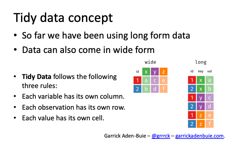
Pivoting data

Not this…

but this!

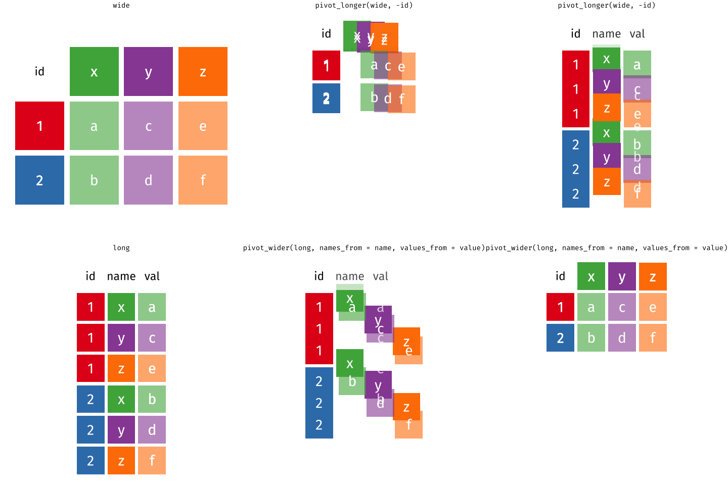
Wider vs. longer

wider more columns ::: {.cell} ::: {.cell-output .cell-output-stdout}

# A tibble: 2 × 4
  customer_id item_1 item_2       item_3
        <dbl> <chr>  <chr>        <chr> 
1           1 bread  milk         banana
2           2 milk   toilet paper <NA>

:::

longer more rows ::: {.cell} ::: {.cell-output .cell-output-stdout}

# A tibble: 6 × 3
  customer_id item_no item        
        <dbl> <chr>   <chr>       
1           1 item_1  bread       
2           1 item_2  milk        
3           1 item_3  banana      
4           2 item_1  milk        
5           2 item_2  toilet paper
6           2 item_3  <NA>

::: ::: :::

`pivot_longer()`

data (as usual)
cols: columns to pivot into longer format
names_to: name of the column where column names of pivoted variables go (character string)
values_to: name of the column where data in pivoted variables go (character string)

pivot_longer(
  data, 
  cols, 
  names_to = "name", #<<
  values_to = "value"
  )

Customers \(\rightarrow\) purchases

purchases <- customers |>
  pivot_longer( #<<
    cols = item_1:item_3,  # variables item_1 to item_3 #<<
    names_to = "item_no",  # column names -> new column called item_no #<<
    values_to = "item"     # values in columns -> new column called item #<<
    ) #<<

purchases

# A tibble: 6 × 3
  customer_id item_no item        
        <dbl> <chr>   <chr>       
1           1 item_1  bread       
2           1 item_2  milk        
3           1 item_3  banana      
4           2 item_1  milk        
5           2 item_2  toilet paper
6           2 item_3  <NA>

Purchases \(\rightarrow\) customers

data (as usual)
names_from: which column in the long format contains the what should be column names in the wide format
values_from: which column in the long format contains the what should be values in the new columns in the wide format

purchases |>
  pivot_wider( #<<
    names_from = item_no, #<<
    values_from = item #<<
  ) #<<

# A tibble: 2 × 4
  customer_id item_1 item_2       item_3
        <dbl> <chr>  <chr>        <chr> 
1           1 bread  milk         banana
2           2 milk   toilet paper <NA>

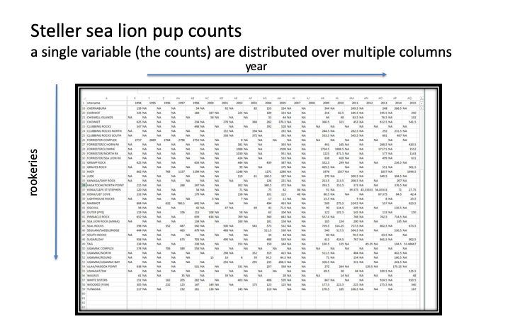
Steller sea lions

We have data on Steller sea lion pup counts over time at a bunch of rookeries in Alaska.

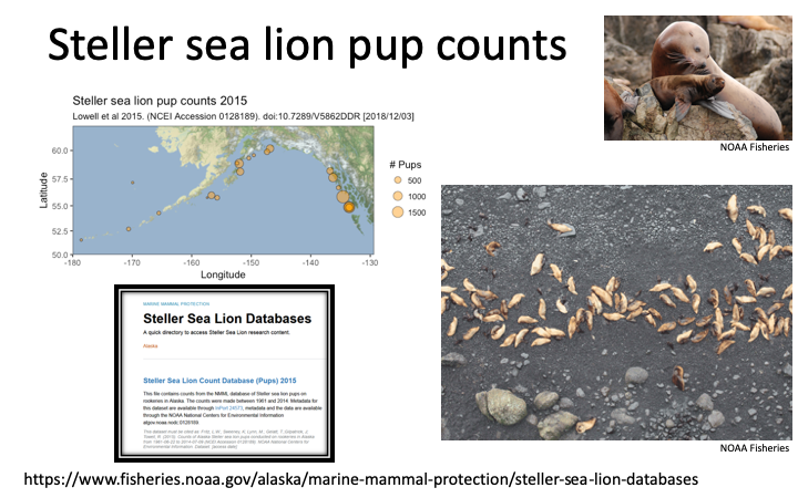
The number of data points for each rookery is not the same.

We want to investigate the annual trend in counts for each rookery.

Lab exercise 3/4 - Sea lion Pups

Read in the data from SSLpupcounts.csv.
Convert the data from wide format to long format.
Print the top 10 rows of the new long format data.
BONUS Convert back to wide format from long format.

05:00

We…

have multiple data frames

want to bring them together

Data: Women in science

Information on 10 women in science who changed the world

name
Ada Lovelace
Marie Curie
Janaki Ammal
Chien-Shiung Wu
Katherine Johnson
Rosalind Franklin
Vera Rubin
Gladys West
Flossie Wong-Staal
Jennifer Doudna

.footnote[ Source: Discover Magazine]

professions

# A tibble: 10 × 2
   name               profession                        
   <chr>              <chr>                             
 1 Ada Lovelace       Mathematician                     
 2 Marie Curie        Physicist and Chemist             
 3 Janaki Ammal       Botanist                          
 4 Chien-Shiung Wu    Physicist                         
 5 Katherine Johnson  Mathematician                     
 6 Rosalind Franklin  Chemist                           
 7 Vera Rubin         Astronomer                        
 8 Gladys West        Mathematician                     
 9 Flossie Wong-Staal Virologist and Molecular Biologist
10 Jennifer Doudna    Biochemist

dates

# A tibble: 8 × 3
  name               birth_year death_year
  <chr>                   <dbl>      <dbl>
1 Janaki Ammal             1897       1984
2 Chien-Shiung Wu          1912       1997
3 Katherine Johnson        1918       2020
4 Rosalind Franklin        1920       1958
5 Vera Rubin               1928       2016
6 Gladys West              1930         NA
7 Flossie Wong-Staal       1947         NA
8 Jennifer Doudna          1964         NA

works

# A tibble: 9 × 2
  name               known_for                                                  
  <chr>              <chr>                                                      
1 Ada Lovelace       first computer algorithm                                   
2 Marie Curie        theory of radioactivity,  discovery of elements polonium a…
3 Janaki Ammal       hybrid species, biodiversity protection                    
4 Chien-Shiung Wu    confim and refine theory of radioactive beta decy, Wu expe…
5 Katherine Johnson  calculations of orbital mechanics critical to sending the …
6 Vera Rubin         existence of dark matter                                   
7 Gladys West        mathematical modeling of the shape of the Earth which serv…
8 Flossie Wong-Staal first scientist to clone HIV and create a map of its genes…
9 Jennifer Doudna    one of the primary developers of CRISPR, a ground-breaking…

Desired output

# A tibble: 10 × 5
   name               profession                 birth_year death_year known_for
   <chr>              <chr>                           <dbl>      <dbl> <chr>    
 1 Ada Lovelace       Mathematician                      NA         NA first co…
 2 Marie Curie        Physicist and Chemist              NA         NA theory o…
 3 Janaki Ammal       Botanist                         1897       1984 hybrid s…
 4 Chien-Shiung Wu    Physicist                        1912       1997 confim a…
 5 Katherine Johnson  Mathematician                    1918       2020 calculat…
 6 Rosalind Franklin  Chemist                          1920       1958 <NA>     
 7 Vera Rubin         Astronomer                       1928       2016 existenc…
 8 Gladys West        Mathematician                    1930         NA mathemat…
 9 Flossie Wong-Staal Virologist and Molecular …       1947         NA first sc…
10 Jennifer Doudna    Biochemist                       1964         NA one of t…

Inputs, reminder

names(professions)

[1] "name"       "profession"

names(dates)

[1] "name"       "birth_year" "death_year"

names(works)

[1] "name"      "known_for"

nrow(professions)

[1] 10

nrow(dates)

[1] 8

nrow(works)

[1] 9

Joining data frames

something_join(x, y)

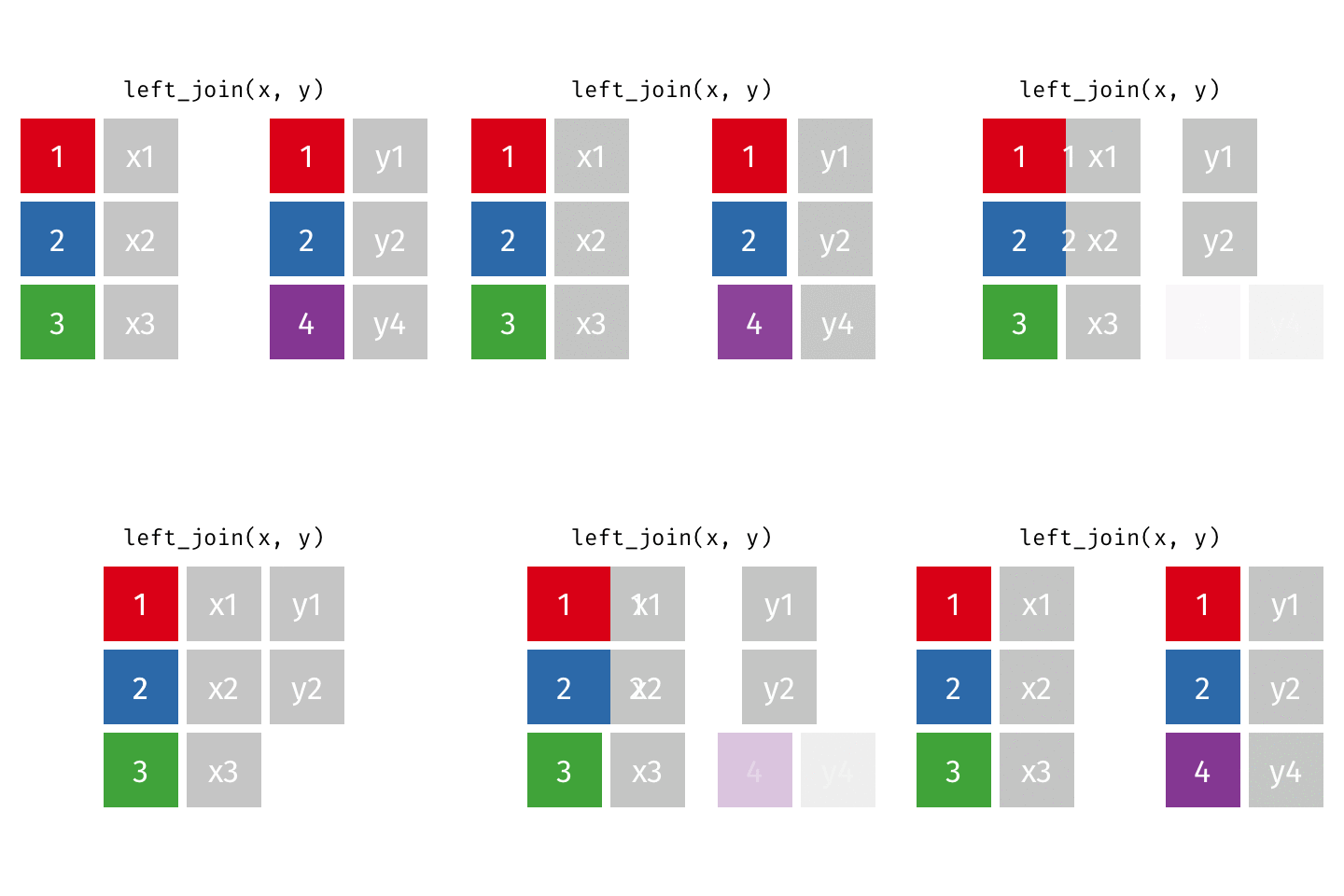
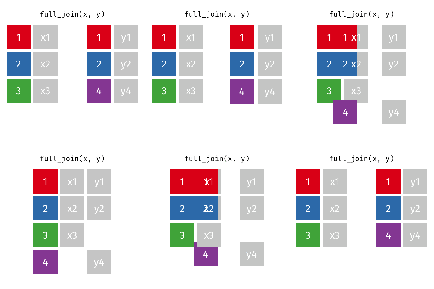
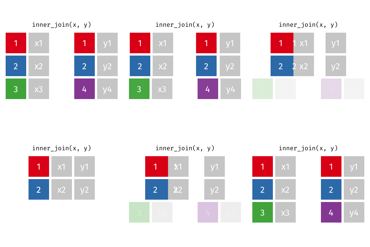
left_join(): all rows from x
right_join(): all rows from y
full_join(): all rows from both x and y
semi_join(): all rows from x where there are matching values in y, keeping just columns from x
inner_join(): all rows from x where there are matching values in y, return all combination of multiple matches in the case of multiple matches
anti_join(): return all rows from x where there are not matching values in y, never duplicate rows of x
…

Setup

For the next few slides…

# A tibble: 3 × 2
     id value_x
  <dbl> <chr>  
1     1 x1     
2     2 x2     
3     3 x3

# A tibble: 3 × 2
     id value_y
  <dbl> <chr>  
1     1 y1     
2     2 y2     
3     4 y4

`left_join()`

left_join(x, y)

# A tibble: 3 × 3
     id value_x value_y
  <dbl> <chr>   <chr>  
1     1 x1      y1     
2     2 x2      y2     
3     3 x3      <NA>

`left_join()`

professions |>
  left_join(dates) #<<

# A tibble: 10 × 4
   name               profession                         birth_year death_year
   <chr>              <chr>                                   <dbl>      <dbl>
 1 Ada Lovelace       Mathematician                              NA         NA
 2 Marie Curie        Physicist and Chemist                      NA         NA
 3 Janaki Ammal       Botanist                                 1897       1984
 4 Chien-Shiung Wu    Physicist                                1912       1997
 5 Katherine Johnson  Mathematician                            1918       2020
 6 Rosalind Franklin  Chemist                                  1920       1958
 7 Vera Rubin         Astronomer                               1928       2016
 8 Gladys West        Mathematician                            1930         NA
 9 Flossie Wong-Staal Virologist and Molecular Biologist       1947         NA
10 Jennifer Doudna    Biochemist                               1964         NA

`right_join()`

right_join(x, y)

# A tibble: 3 × 3
     id value_x value_y
  <dbl> <chr>   <chr>  
1     1 x1      y1     
2     2 x2      y2     
3     4 <NA>    y4

`right_join()`

professions |>
  right_join(dates) #<<

# A tibble: 8 × 4
  name               profession                         birth_year death_year
  <chr>              <chr>                                   <dbl>      <dbl>
1 Janaki Ammal       Botanist                                 1897       1984
2 Chien-Shiung Wu    Physicist                                1912       1997
3 Katherine Johnson  Mathematician                            1918       2020
4 Rosalind Franklin  Chemist                                  1920       1958
5 Vera Rubin         Astronomer                               1928       2016
6 Gladys West        Mathematician                            1930         NA
7 Flossie Wong-Staal Virologist and Molecular Biologist       1947         NA
8 Jennifer Doudna    Biochemist                               1964         NA

`full_join()`

full_join(x, y)

# A tibble: 4 × 3
     id value_x value_y
  <dbl> <chr>   <chr>  
1     1 x1      y1     
2     2 x2      y2     
3     3 x3      <NA>   
4     4 <NA>    y4

`full_join()`

dates |>
  full_join(works) #<<

# A tibble: 10 × 4
   name               birth_year death_year known_for                           
   <chr>                   <dbl>      <dbl> <chr>                               
 1 Janaki Ammal             1897       1984 hybrid species, biodiversity protec…
 2 Chien-Shiung Wu          1912       1997 confim and refine theory of radioac…
 3 Katherine Johnson        1918       2020 calculations of orbital mechanics c…
 4 Rosalind Franklin        1920       1958 <NA>                                
 5 Vera Rubin               1928       2016 existence of dark matter            
 6 Gladys West              1930         NA mathematical modeling of the shape …
 7 Flossie Wong-Staal       1947         NA first scientist to clone HIV and cr…
 8 Jennifer Doudna          1964         NA one of the primary developers of CR…
 9 Ada Lovelace               NA         NA first computer algorithm            
10 Marie Curie                NA         NA theory of radioactivity,  discovery…

`inner_join()`

inner_join(x, y)

# A tibble: 2 × 3
     id value_x value_y
  <dbl> <chr>   <chr>  
1     1 x1      y1     
2     2 x2      y2

`inner_join()`

dates |>
  inner_join(works) #<<

# A tibble: 7 × 4
  name               birth_year death_year known_for                            
  <chr>                   <dbl>      <dbl> <chr>                                
1 Janaki Ammal             1897       1984 hybrid species, biodiversity protect…
2 Chien-Shiung Wu          1912       1997 confim and refine theory of radioact…
3 Katherine Johnson        1918       2020 calculations of orbital mechanics cr…
4 Vera Rubin               1928       2016 existence of dark matter             
5 Gladys West              1930         NA mathematical modeling of the shape o…
6 Flossie Wong-Staal       1947         NA first scientist to clone HIV and cre…
7 Jennifer Doudna          1964         NA one of the primary developers of CRI…

Putting it altogether

professions |>
  left_join(dates) |>
  left_join(works)

# A tibble: 10 × 5
   name               profession                 birth_year death_year known_for
   <chr>              <chr>                           <dbl>      <dbl> <chr>    
 1 Ada Lovelace       Mathematician                      NA         NA first co…
 2 Marie Curie        Physicist and Chemist              NA         NA theory o…
 3 Janaki Ammal       Botanist                         1897       1984 hybrid s…
 4 Chien-Shiung Wu    Physicist                        1912       1997 confim a…
 5 Katherine Johnson  Mathematician                    1918       2020 calculat…
 6 Rosalind Franklin  Chemist                          1920       1958 <NA>     
 7 Vera Rubin         Astronomer                       1928       2016 existenc…
 8 Gladys West        Mathematician                    1930         NA mathemat…
 9 Flossie Wong-Staal Virologist and Molecular …       1947         NA first sc…
10 Jennifer Doudna    Biochemist                       1964         NA one of t…

–>

–> –> –> –> –> –>

Exercise 4/4 Sea lion Rookery Counts

SSL_Sites.csv contains the latitude and longitude of sea lion rookeries.
Use a suitable join function to add the lat/lon information and geographic region to the counts dataset.
Summarize the average annual pups that were counted between 2000-2015 in the Aleutian Islands (west of longitude 160W), the Gulf of Alaska (east of longitude 160W, west of 140W), and Southeast Alaska (South of latiutude 60 degrees N, but not in the Pacific Northwest).
BONUS Look up how to make a map using ggplot() to map the rookery counts in 2015.

–>

–> –> –> –> –> –> –> –> –>

–>

–> –> –>

–>

–> –> –> –> –> –> –> –> –> –> –> –> –> –> –> –>

–>

–> –> –> –> –> –> –> –> –>

MAR 536: Lab 4

Lab schedule

Today

setup

Generalized linear modeling

Generalized linear modeling

The glm() function

The glm() function

Poisson regression

RIKZ example

summary(RIKZ_poisson)

broom::augment()

Observed and fitted values for Poisson RIKZ

fitting the GLM in the ggplot call

Lab Exercise 1/4: RIKZ Poisson GLMs

dplyr::case_when()

dplyr::case_when()

dplyr::case_when()

Exercise 2/4

Pivoting data

Not this…

but this!

Wider vs. longer

pivot_longer()

Customers \(\rightarrow\) purchases

Purchases \(\rightarrow\) customers

Steller sea lions

Lab exercise 3/4 - Sea lion Pups

We…

Data: Women in science

Inputs

Desired output

Inputs, reminder

Joining data frames

Joining data frames

Setup

left_join()

left_join()

right_join()

right_join()

full_join()

full_join()

inner_join()

inner_join()

Putting it altogether

Exercise 4/4 Sea lion Rookery Counts

The `glm()` function

The `glm()` function

`summary(RIKZ_poisson)`

`broom::augment()`

`pivot_longer()`

`left_join()`

`left_join()`

`right_join()`

`right_join()`

`full_join()`

`full_join()`

`inner_join()`

`inner_join()`