Biological Stats 2: Lab 1

Dr. Gavin Fay

01/18/2023

Lab schedule

1/18: Introduction to R and R Studio, working with data
1/25: Intro to Visualization
2/01: Probability, linear modeling
2/08: Data wrangling, model summaries
2/15: Iteration
2/22: Creating functions, debugging
3/01: Simulation, Resampling
3/15: Flex: more modeling (brms, glmmTMB)
3/29: Spatial data or tidymodeling

Format for lab component

Description/overview of concepts by instructor
Live coding. Interactive, follow along yourselves
Lab exercises to practice material
Assignment each week is to finish the exercises
Extra credit: #TidyTuesday
Community support
“Try stuff and see what happens”

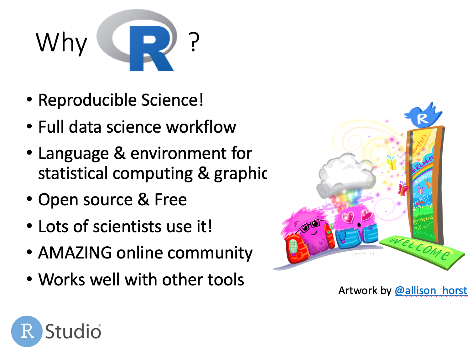
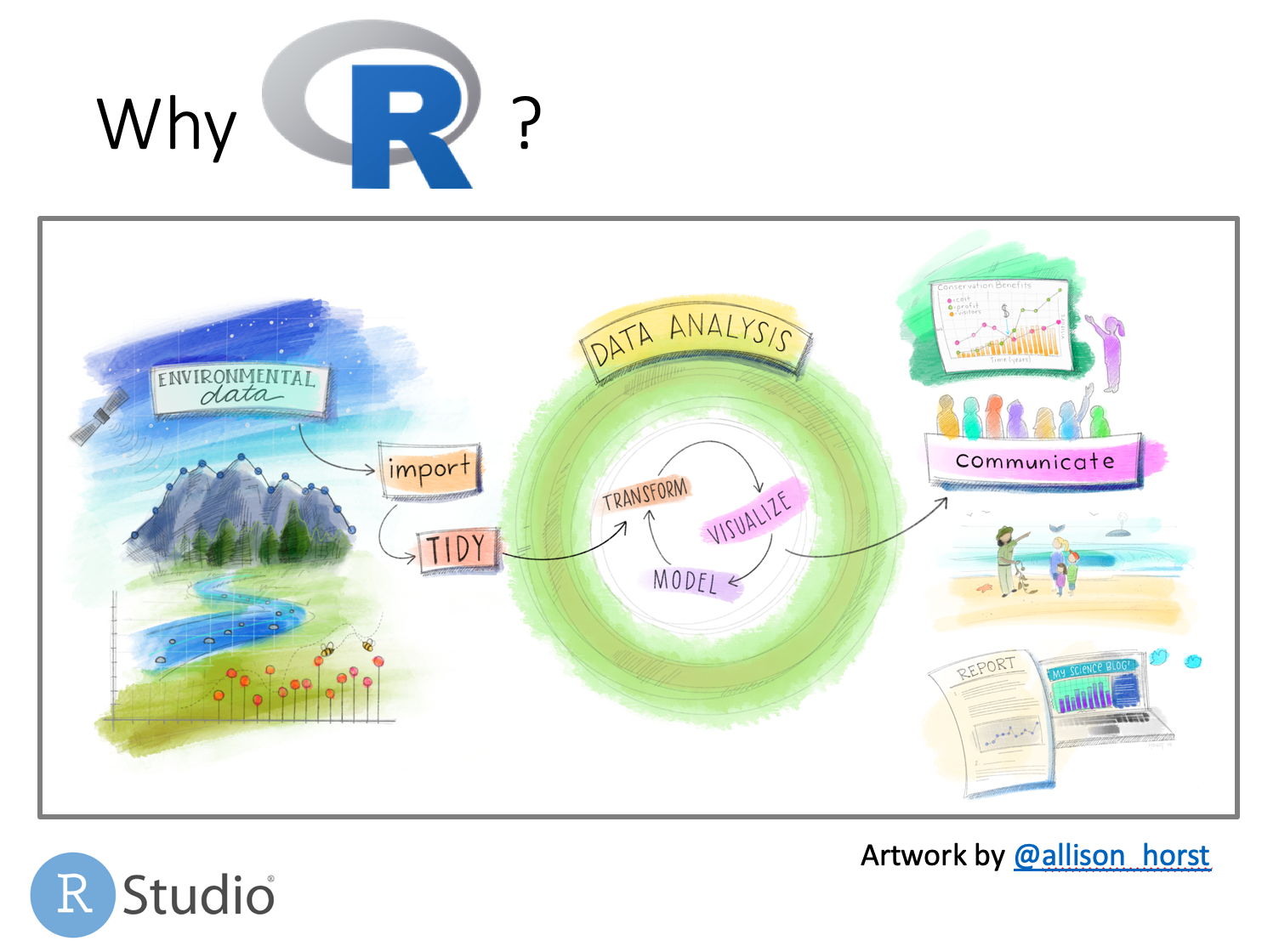
Why R?

Reproducible
- command line interface encourages organization
- scripts allow others (and you!) to reproduce analyses from end-to-end
- integration of analysis with document creation

Extensible
- new methods delivered as developed
- continual expansion through new packages

Open-source
- all code can be examined by the user

Free
- available to large set of users (and therefore developers)

R is not the only solution out there.
The real goal is not to teach R, but concepts that all programming depends on.

Trevor Branch rule:

“Every analysis you do on a dataset will have to be redone 10–15 times before publication. Plan accordingly.”

Reproducibility checklist

What does it mean for a data analysis to be “reproducible”?

Near-term goals:

Are the tables and figures reproducible from the code and data?
Does the code actually do what you think it does?
In addition to what was done, is it clear why it was done?

Long-term goals:

Can the code be used for other data?
Can you extend the code to do other things?

Toolkit for reproducibility

Scriptability $\rightarrow$ R
Literate programming (code, narrative, output in one place) $\rightarrow$ R Markdown
Version control $\rightarrow$ Git / GitHub

R and RStudio

R is an open-source statistical programming language
R is also an environment for statistical computing and graphics
It’s easily extensible with packages

RStudio is a convenient interface for R called an IDE (integrated development environment), e.g. “I write R code in the RStudio IDE”
RStudio is not a requirement for programming with R, but it’s very commonly used by R programmers and data scientists

Using R today: RStudio Cloud

An alternative:

web browser interface https://posit.cloud/content/5243518

R packages

Packages are the fundamental units of reproducible R code. They include reusable R functions, the documentation that describes how to use them, and sample data ¹
As of September 2020, there are over 16,000 R packages available on CRAN (the Comprehensive R Archive Network)²
We’re going to work with a small (but important) subset of these!

Tour: R and RStudio

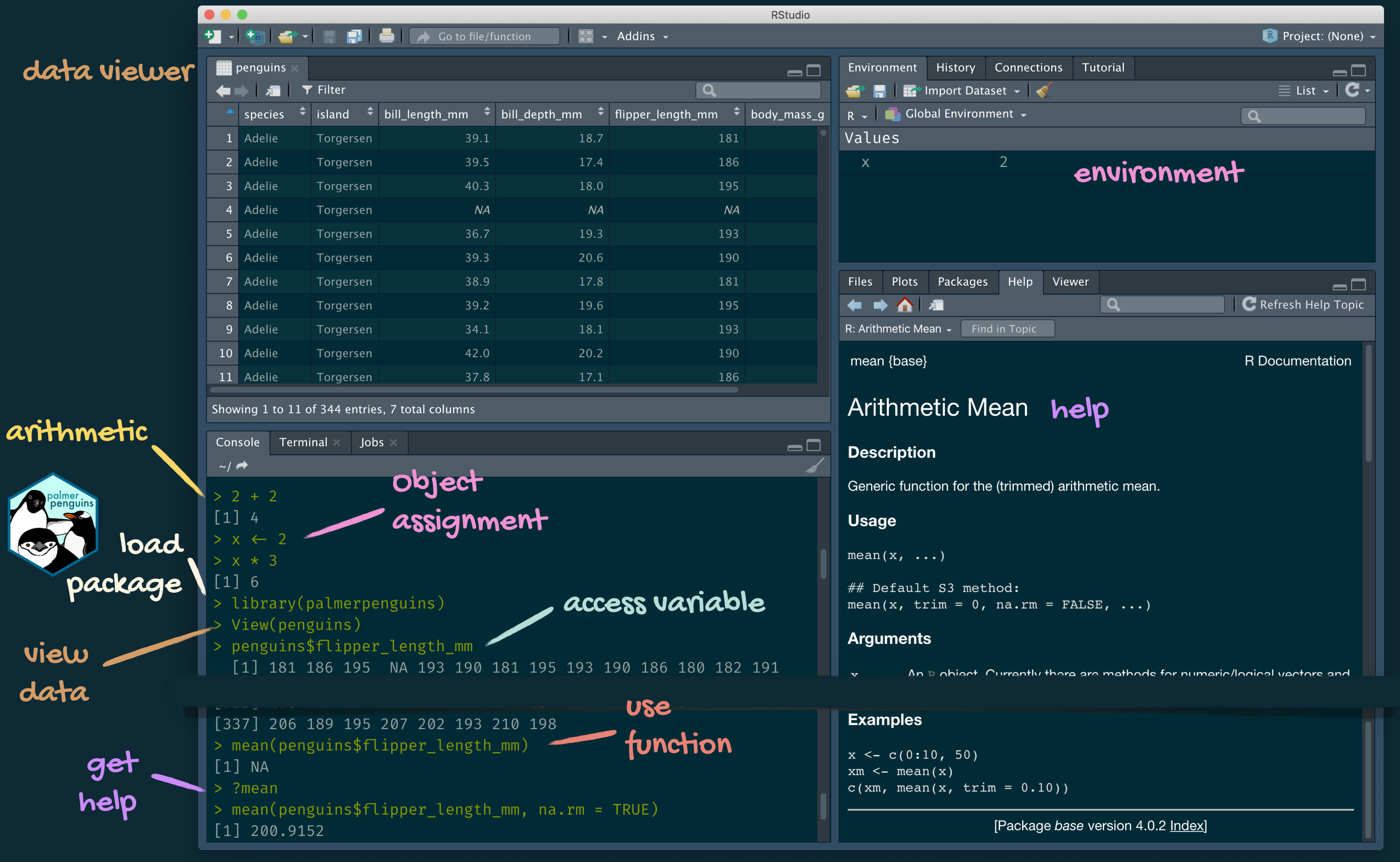
A short list (for now) of R essentials

Functions are (most often) verbs, followed by what they will be applied to in parentheses:

do_this(to_this)
do_that(to_this, to_that, with_those)

Packages are installed with the install.packages function and loaded with the library function, once per session:

install.packages("package_name")
library(package_name)

tidyverse

tidyverse.org

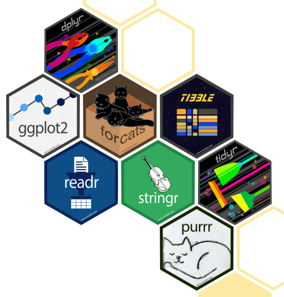
The tidyverse is an opinionated collection of R packages designed for data science
All packages share an underlying philosophy and a common grammar

Getting started

Enter instructions at R console command line prompt (>): e.g. type

2 + 2

R acts as a calculator and returns (prints) the result.

2 + 2
[1] 4

Simple commands

3^2
[1] 9
2*(2+2)
[1] 8
2*2+2
[1] 6
log(10)
[1] 2.302585
exp(1)
[1] 2.718282
x <- 3
2*x
[1] 6

The <- means ‘assign’. i.e. ‘assign a value of 3 to the variable x’. <- is preferable to using =

Scripts and RStudio

Typing commands into the console can get tedious.
Scripts are text files containing lines of code.
Scripts provide a complete record of analyses.
Code can be run (executed) from these files repeatedly.
Scripts can be created in a text editor and copied into the R console.

Or…

RStudio integrates scripts, R console, and output in a user-friendly development environment.
To run code in RStudio, select code and type
Ctrl+Enter (Windows)
Command+Enter (Mac)
The code will run in the R console.

rmarkdown

rmarkdown.rstudio.com

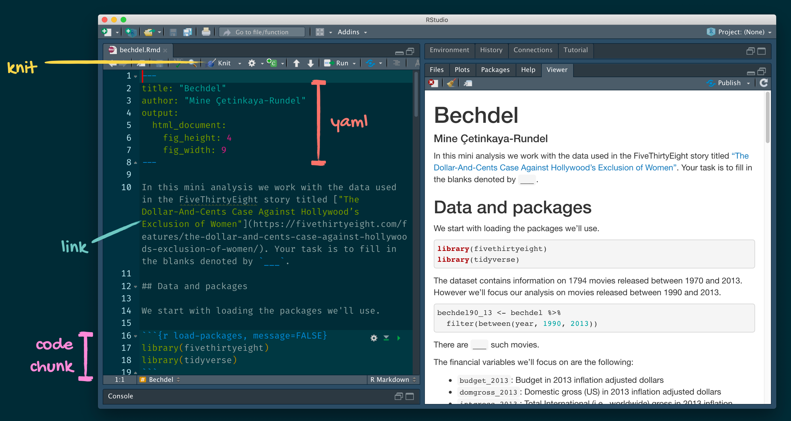
rmarkdown and the various packages that support it enable R users to write their code and prose in reproducible computational documents
We will generally refer to R Markdown documents (with .Rmd extension), e.g. “Do this in your R Markdown document” and rarely discuss loading the rmarkdown package

R Markdown

Fully reproducible reports – each time you knit the analysis is ran from the beginning
Simple markdown syntax for text
Code goes in chunks, defined by three backticks, narrative goes outside of chunks

Tour: R Markdown

Getting Help in R

R is a programming language, there is a learning curve.

Fortunately, there are lots of resources:

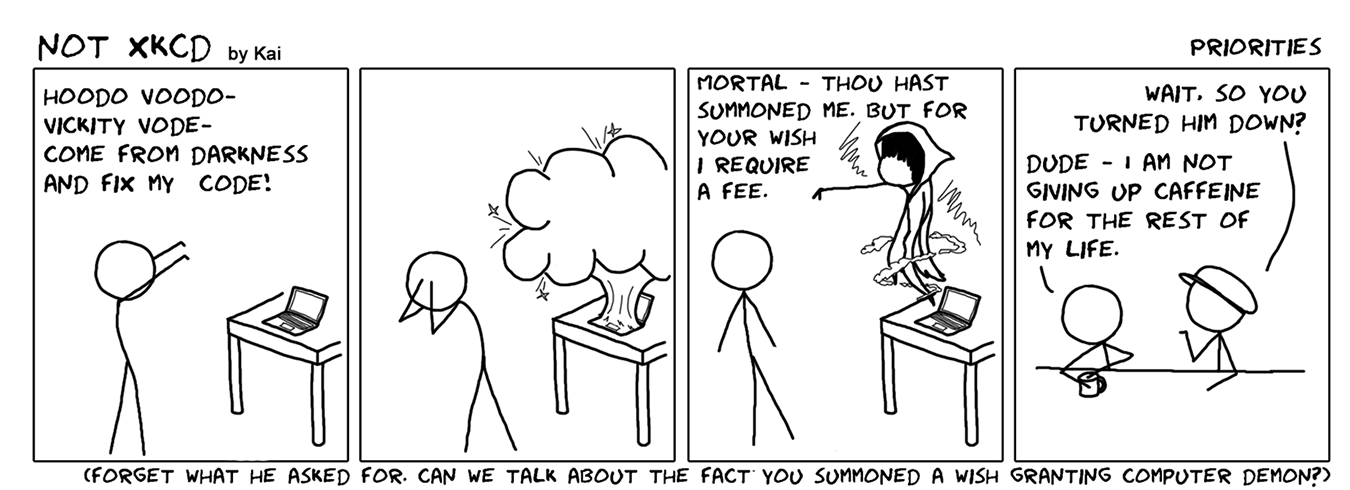
Don’t summon a wish-granting computer demon.

Getting Help in R

R is a programming language, there is a learning curve.

Fortunately, there are lots of resources:
- help files
- online search results
- books
- colleagues
- RStudio Community

?(mean)
help("mean")

The above both get help for the function mean.
Use help.search("function.name") to search across packages.

str(object.name) shows the structure of an object.

R Help files (`?mean`)

Common format:

Description (what the function does)
Usage (how to use it)
Arguments (what the function needs, options)
Value (what does the function return)
See Also (related functions)
Examples (sample code showing how the function works)

Read function documentation and explore behavior by running examples!

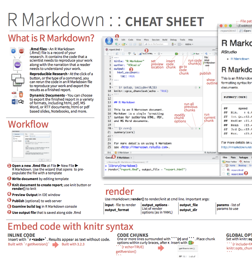
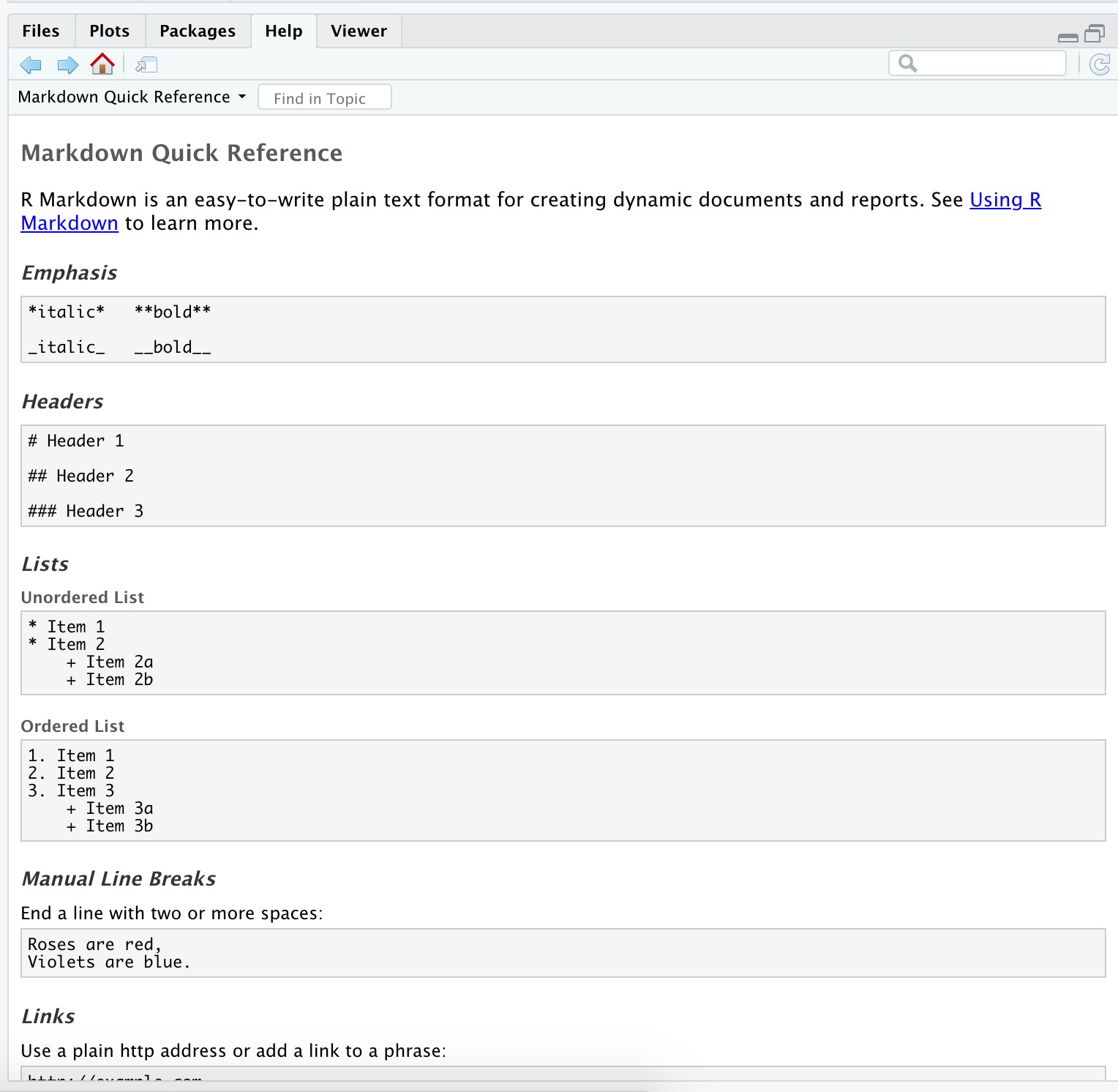
R Markdown help

R Markdown Cheat Sheet
Help -> Cheatsheets

Markdown Quick Reference
Help -> Markdown Quick Reference

Projects in RStudio

Good to keep all the files associated with a particular project organized together – input data, R scripts, analytical results, figures.

RStudio has built-in support for this via its projects.

Projects provide an easy organization of your files and analyses.

R runs from a working directory, the location (folder) on your computer that R will use as a default when looking for data files, producing output, etc.

Project files (.Rproj)

When you open a project, RStudio sets the working directory to the folder in which the .Rproj file exists.

Using projects can be VERY helpful.

Lab exercise 1/4

(Instructions also in lab-exercise-01.pdf)

Start a new project. (call it biostats2 or something similar)
Open a new R markdown file. Save it. (name it lastname_lab1.Rmd or something similar)
At the top of the script, add comments with your name and lab 1.
Work in pairs or individually.
Submit your .Rmd file via myCourses before lab next week.

Write code that evaluates the following when run. \[7 + 5(4+3)\] \[e^{-5(0.2+0.15)}\] \[\frac{\sqrt{1+2(3+2)}}{\ln(3^2+2)}\]

Objects

Common types of objects
- Numbers
- Characters (i.e. text or strings)
- Tables
- Vectors and matrices
- Plots
- Statistical output
- Functions

Objects in R are global

Viewing objects: In RStudio see top-right Workspace tab
More generally:

  print(myobject)
  myobject

ls() lists all objects in the workspace.
Use rm() to remove an object.

Data types (modes)

Describe how objects are stored in computer memory.

In R you do not need to specify the data type.

Common data types:

Numeric (integer, floating point numbers or doubles)
Logical (Boolean, true or false)
Characters (text or string data)

Types are not always obvious in R, but can be important to know.

Data types II

myobject <- log(10)
mode(myobject)
[1] "numeric"
is.numeric(myobject)
[1] TRUE
typeof(myobject)
[1] "double"
newobject <- as.integer(myobject)
typeof(newobject)
[1] "integer"
is.character(myobject)
[1] FALSE
typeof("hello world")
[1] "character"

Vectors

weights <- c(2.3,5.4,7.5,9)
print(weights)
[1] 2.3 5.4 7.5 9.0
years <- 2007:2016
print(years)
 [1] 2007 2008 2009 2010 2011 2012 2013 2014 2015 2016
years <- seq(from=2000,to=2016,by=2)
print(years)
[1] 2000 2002 2004 2006 2008 2010 2012 2014 2016
x <- rep(3,times=10)
print(x)
 [1] 3 3 3 3 3 3 3 3 3 3
rep(1:3,times=3)
[1] 1 2 3 1 2 3 1 2 3
rep(1:3,length=10)
 [1] 1 2 3 1 2 3 1 2 3 1

More on Vectors

Vectors are ordered and can be referred to by element(s) using [ ]

(years <- 2007:2016)
 [1] 2007 2008 2009 2010 2011 2012 2013 2014 2015 2016
years[3]
[1] 2009
years[5:6]
[1] 2011 2012
which(years==2010)
[1] 4
years[-c(2,4)] # A negative index excludes elements
[1] 2007 2009 2011 2012 2013 2014 2015 2016

Vector operations are element-wise

(x <- 1:5)
[1] 1 2 3 4 5
2*x
[1]  2  4  6  8 10

Lab exercise 2/4

(Instructions also in lab-exercise-01.pdf)

Create vectors using seq(), rep(), and mathematical operators. Only use c() when absolutely necessary.
hint Remember you can get help on a function by typing ?functionname

Positive integers from 1 to 99
Odd integers between 1 and 99
The numbers 1,1,1, 2,2,2, 3,3,3
The numbers -5,-4,-3,-5,-4,-3,-5,-4,-3
The fractions 1, 1/2, 1/3, 1/4, …, 1/10
The cubes 1, 8, 27, 64, 125, 216

Useful functions

x <- c(5,3,2,6,3,9,1,18)
length(x)  # length of vector x
[1] 8
sort(unique(x))  # sorted vector of unique values in x
[1]  1  2  3  5  6  9 18
min(x)     # minimum value in x
[1] 1
max(x)     # maximum value in x
[1] 18
mean(x)    # mean of x
[1] 5.875
median(x)  # median of x
[1] 4
sd(x)      # standard deviation of x
[1] 5.514591
range(x)   # range of values in x
[1]  1 18
range(x)[2]  # 2nd element of values returned by range()
[1] 18
quantile(x) # optional argument 'probs' can be handy
   0%   25%   50%   75%  100% 
 1.00  2.75  4.00  6.75 18.00

Boolean logic operators

Operator	R Code
AND	& (&&)
OR	\| (\|\|)
NOT	!
less than	<
greater than	>
less than or equal	<=
greater than or equal	>=
equals	==
NOT equal	!=

&& and || are used when asking IF statements.
These only use a single value, not a vector.

Boolean examples

x <- 7 
x == 7 
[1] TRUE
x < 10 
[1] TRUE
x < -3 
[1] FALSE
x > 0 & x <= 12
[1] TRUE
x >= 10 | x < 0 
[1] FALSE

y <- c(4,8)
y > 5   #returns a logical vector
[1] FALSE  TRUE
y[y>5]  #returns elements of y that meet condition
[1] 8
which(y>5) #index of y that meets condition
[1] 2
any(y>5)
[1] TRUE
all(y>5)
[1] FALSE

Lab exercise 3/4

Complete the following using the vector y:

y <- c(3,2,15,-1,22,1,9,17,5)

Display the first and last values.
Find the last value for a vector of any length.
Display the values that are greater than the mean of y.
Display the positions (indices) of the values greater than the mean.
Are all the values positive?
Are any of the values equal to the mean?
Are any of the values equal to the median?

Other types of objects

matrices (more generally, arrays)
- multi-dimensional generalizations of vectors.
- are vectors that can be indexed by two or more indices.

factors
- compact ways to handle categorical data.

lists
- general form of vector, elements need not be the same type.
- elements often themselves vectors or lists.
- convenient way to return results of statistical computations.

dataframes
- matrix-like structures, columns can be of different types.
- often ‘data matrices’ with one row per observational unit but with (possibly) both numerical and categorical variables.

functions
- are themselves objects in R which can be stored in the project’s workspace.
- provide a simple and convenient way to extend R.

Dataframes

There are lots of data set examples in R.
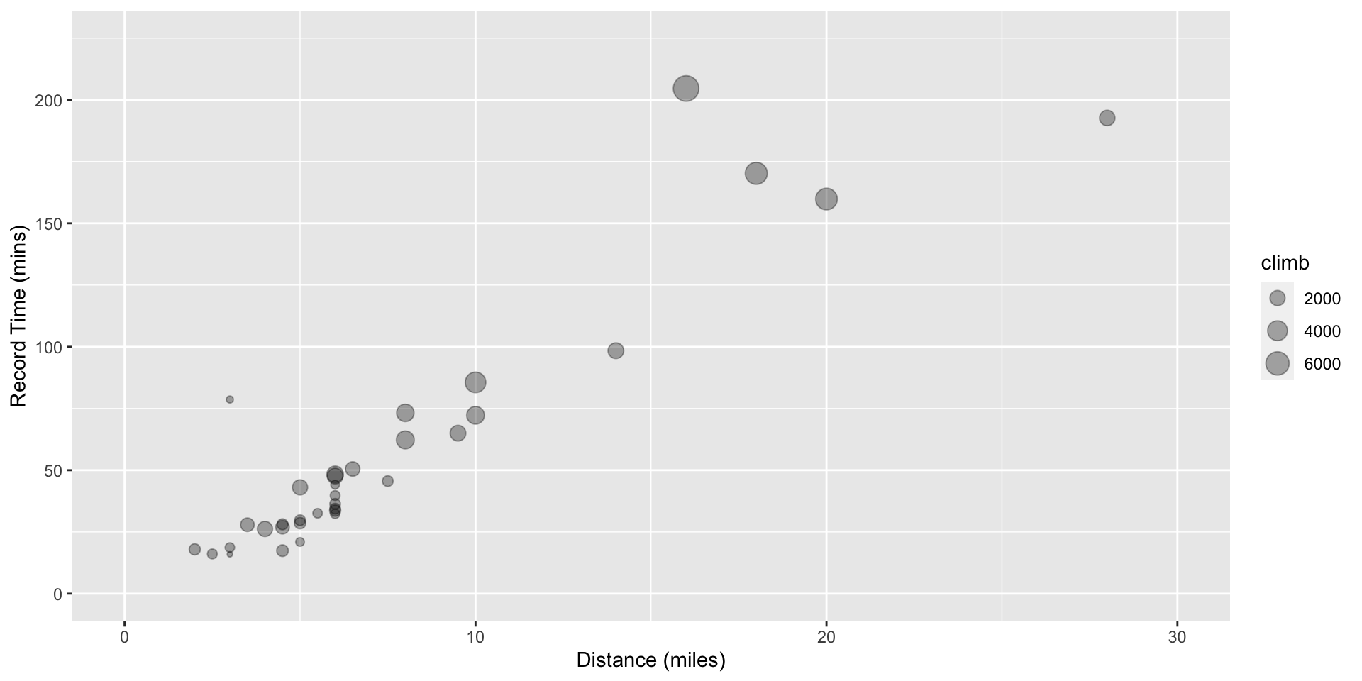
e.g. record times for 35 Scottish hill races

library(MASS)
head(hills,n=3) # shows first few lines. Also tail()
             dist climb   time
Greenmantle   2.5   650 16.083
Carnethy      6.0  2500 48.350
Craig Dunain  6.0   900 33.650
names(hills)  # get the names of the data frame
[1] "dist"  "climb" "time"

Creating dataframes

fish <- c("cod","haddock","dogfish","pollock")
length <- c(34,23,75,18)
age <- c(6,3,17,2)
fish.data <- data.frame(fish=fish,length=length,age=age)
head(fish.data)
     fish length age
1     cod     34   6
2 haddock     23   3
3 dogfish     75  17
4 pollock     18   2

Extracting information from data frames

Use the $ to extract vectors from a data frame

hills$dist
 [1]  2.5  6.0  6.0  7.5  8.0  8.0 16.0  6.0  5.0  6.0 28.0  5.0  9.5  6.0  4.5
[16] 10.0 14.0  3.0  4.5  5.5  3.0  3.5  6.0  2.0  3.0  4.0  6.0  5.0  6.5  5.0
[31] 10.0  6.0 18.0  4.5 20.0

You can also specify the row index, column index, or both object[row,column]

# extract the element in row 1, column 2
hills[1,2]
[1] 650
hills$climb[1]
[1] 650
# extract the first row
hills[1,]
            dist climb   time
Greenmantle  2.5   650 16.083

# extract all of column 2
hills[,2]   # also hills[,"climb"]
 [1]  650 2500  900  800 3070 2866 7500  800  800  650 2100 2000 2200  500 1500
[16] 3000 2200  350 1000  600  300 1500 2200  900  600 2000  800  950 1750  500
[31] 4400  600 5200  850 5000
# exclude column 1, but retain the other columns (1st 3 rows)
hills[1:3,-1]  
             climb   time
Greenmantle    650 16.083
Carnethy      2500 48.350
Craig Dunain   900 33.650
# extract rows 4 and 7
hills[c(4,7),]
             dist climb    time
Ben Rha       7.5   800  45.600
Bens of Jura 16.0  7500 204.617
# extract the rows that are specified by the object x
x <- c(4,7,nrow(hills))
hills[x,]
             dist climb    time
Ben Rha       7.5   800  45.600
Bens of Jura 16.0  7500 204.617
Moffat Chase 20.0  5000 159.833

Extracting information from data frames (2)

Data frames are commonly used in a structure called a ‘tibble’, from the tidyverse.

#install.packages('tidyverse')
library(tidyverse)

hills_tbl <- as_tibble(hills)
hills_tbl
# A tibble: 35 × 3
    dist climb  time
   <dbl> <int> <dbl>
 1   2.5   650  16.1
 2   6    2500  48.4
 3   6     900  33.6
 4   7.5   800  45.6
 5   8    3070  62.3
 6   8    2866  73.2
 7  16    7500 205. 
 8   6     800  36.4
 9   5     800  29.8
10   6     650  39.8
# … with 25 more rows

Extract variables using the select verb function in the dplyr package

dplyr::select(hills,dist)
                 dist
Greenmantle       2.5
Carnethy          6.0
Craig Dunain      6.0
Ben Rha           7.5
Ben Lomond        8.0
Goatfell          8.0
Bens of Jura     16.0
Cairnpapple       6.0
Scolty            5.0
Traprain          6.0
Lairig Ghru      28.0
Dollar            5.0
Lomonds           9.5
Cairn Table       6.0
Eildon Two        4.5
Cairngorm        10.0
Seven Hills      14.0
Knock Hill        3.0
Black Hill        4.5
Creag Beag        5.5
Kildcon Hill      3.0
Meall Ant-Suidhe  3.5
Half Ben Nevis    6.0
Cow Hill          2.0
N Berwick Law     3.0
Creag Dubh        4.0
Burnswark         6.0
Largo Law         5.0
Criffel           6.5
Acmony            5.0
Ben Nevis        10.0
Knockfarrel       6.0
Two Breweries    18.0
Cockleroi         4.5
Moffat Chase     20.0

Create a new variable of the race names

  hills_tbl <- mutate(hills_tbl,race=rownames(hills))
  hills_tbl <- dplyr::select(hills_tbl,race,everything())
  hills_tbl
# A tibble: 35 × 4
   race          dist climb  time
   <chr>        <dbl> <int> <dbl>
 1 Greenmantle    2.5   650  16.1
 2 Carnethy       6    2500  48.4
 3 Craig Dunain   6     900  33.6
 4 Ben Rha        7.5   800  45.6
 5 Ben Lomond     8    3070  62.3
 6 Goatfell       8    2866  73.2
 7 Bens of Jura  16    7500 205. 
 8 Cairnpapple    6     800  36.4
 9 Scolty         5     800  29.8
10 Traprain       6     650  39.8
# … with 25 more rows

Quickly visualize the dataset

library(ggplot2)
ggplot(data = hills_tbl, mapping = aes(x=dist,y=time)) +
  geom_point(aes(size = climb), alpha = 1/3) +
  xlab("Distance (miles)") +
  ylab("Record Time (mins)") +
  xlim(0,30) + ylim(0,225)

Extracting elements logically

fish <- c("cod","haddock","dogfish","pollock")
length <- c(34,23,75,18)
age <- c(6,3,17,2)
fish_data <- tibble(fish=fish,length=length,age=age)
fish_data$age   # a vector
[1]  6  3 17  2
fish_data$age > 5  # a logical vector
[1]  TRUE FALSE  TRUE FALSE
filter(fish_data, age>5) #avoids having to create a logical vector
# A tibble: 2 × 3
  fish    length   age
  <chr>    <dbl> <dbl>
1 cod         34     6
2 dogfish     75    17
# combining conditions
filter(fish_data, age > 5, fish == "dogfish")
# A tibble: 1 × 3
  fish    length   age
  <chr>    <dbl> <dbl>
1 dogfish     75    17
filter(fish_data, length < 25 | length >= 50)
# A tibble: 3 × 3
  fish    length   age
  <chr>    <dbl> <dbl>
1 haddock     23     3
2 dogfish     75    17
3 pollock     18     2

Using the Pipe

Combine verb operations with the pipe operator (|>) e.g.

fish_data |>
  mutate(weight = (length/100)^3) |>
  filter(age > 5)
# A tibble: 2 × 4
  fish    length   age weight
  <chr>    <dbl> <dbl>  <dbl>
1 cod         34     6 0.0393
2 dogfish     75    17 0.422

The pipe passes the result from one function call to the next.
Can be read as “and then”.
(also the older tidyverse pipe: %>% )

Summarizing Data

After selecting data we might like to perform analyses on it.
We can use group_by() to recognize structure in the data.
Then apply functions to variables using summarize()
Recall gapminder data, find the average life expectancy in 2007 for each continent

#install.packages('gapminder')
library(gapminder)
gapminder |> 
  filter(year == 2007) |> 
  group_by(continent) |>
  summarize(avg_lifeExp = mean(lifeExp))
# A tibble: 5 × 2
  continent avg_lifeExp
  <fct>           <dbl>
1 Africa           54.8
2 Americas         73.6
3 Asia             70.7
4 Europe           77.6
5 Oceania          80.7

Tips and Tricks

Comments
Use comments within R code to document the purpose of your code. Anything on a line after a # is ignored by R. RStudio uses a different color to help readability.

SAVE your scripts(!), not workspaces. Use meaningful variable names. Adopt a coding style and use consistently.
(e.g. https://google.github.io/styleguide/Rguide.xml)

The str() function can be incredibly helpful when querying objects.

Make use of help() documentation.

There are almost always multiple ways of getting the same result.
We’ll mostly use low level functions to help you understand how R works.
Some advanced functions are cleaner and do things more quickly.

Lab exercise 4/4 (data frames using `hills`)

Display the first 5 rows of the hills dataframe.
Find the fastest time.
Display the hill races (and distance, climbs, and times) with the 3 fastest times.
Extract and display the record time for Cairngorm.
Find how many hill races have a climb greater than the mean.
Display the names of the hill races that have a climb greater than the mean.
Display the names and times of the races that are at least 10 miles long and have a climb greater than 4000 feet.
Find the standard deviation of the record times for all races except for the highest climb, the Bens of Jura.
Display the range (minimum and maximum) of the average speed for the races.
Find the race that had the fastest average speed.
BONUS Find the mean of the record times for races whose names start with letters A through K.

Next time…

1/18: Introduction to R and R Studio, working with data
1/25: Intro to Vizualization
2/01: Probability, linear modeling
2/08: Data wrangling, model summaries
2/15: Iteration
2/22: Creating functions, debugging
3/01: Simulation, Resampling
3/15: Flex: more modeling (brms, glmmTMB)
3/29: Spatial data or tidymodeling

Biological Stats 2: Lab 1

Lab schedule

Format for lab component

Why R?

Recommended reading

Recommended reading

Reproducibility checklist

Toolkit for reproducibility

R and RStudio

Using R today: RStudio Cloud

R packages

Tour: R and RStudio

A short list (for now) of R essentials

tidyverse

Getting started

Simple commands

Scripts and RStudio

rmarkdown

R Markdown

Tour: R Markdown

Getting Help in R

Getting Help in R

R Help files (?mean)

R Markdown help

Projects in RStudio

Lab exercise 1/4

Objects

Data types (modes)

Data types II

Vectors

More on Vectors

Lab exercise 2/4

Useful functions

Boolean logic operators

Boolean examples

Lab exercise 3/4

Other types of objects

Dataframes

Extracting information from data frames

Extracting information from data frames (2)

Quickly visualize the dataset

Extracting elements logically

Using the Pipe

Summarizing Data

Tips and Tricks

Lab exercise 4/4 (data frames using hills)

Next time…

R Help files (`?mean`)

Lab exercise 4/4 (data frames using `hills`)